
Grid Data - Kriging
Gridding refers to the process of interpolating data onto an equally spaced “grid” of cells in a specified coordinate system. For an introduction to gridding and a summary of the different gridding methods click here.
Kriging
Kriging is a geostatistical gridding technique for random data, non-parallel line data, or orthogonal line data. Use the kriging method (KRIGRID) if the data is not sampled along lines that run roughly in the same direction, it is variable between sample locations, known to be statistical in nature, poorly sampled, or clustered. The method is ideally suited to geochemical or other geological sample-based data; it is rarely used with geophysical data, which tends to follow a natural smooth surface.
The Kriging algorithm determines the most probable value at each grid node based on a statistical analysis of the entire data set. For an overview of the method click here.
To perform kriging, you must supply a data channel, an output grid name and optionally the grid cell size. In addition, you also have a variety of options, including the ability to:
-
estimate the average error of the data at each grid node (nugget) and save it to an error grid file.
-
define the grid coverage (spatial limits of the area to be gridded).
-
grid the original data or its logarithmic representation (using cutoffs or a data range).
-
specify desampling values (for low-pass filtering) and a blanking distance (for removing values beyond a certain distance).
-
apply trend removal.
-
choose from multiple variogram models (power, spherical, Gaussian, or exponential).
-
specify the level at which the variogram becomes uncorrelated (sill) and the distance (range) at which the variogram model meets the sill.
Kriging outputs consist of a grid, an error grid and a kriging report (krigrid.log) file. The error grid contains the standard deviation of the estimation at each grid node. The report gives details about the input data, the parameters that were used for processing, and the calculated and model variogram and grid parameters. See Application Notes below for more details.
Use the Grid Data option from the Grid and Image > Gridding menu to grid geostatistical data using the kriging algorithm.
Kriging – Gridding Options
|
Data to grid |
Select the database channel to grid. To specify an array element, append to the channel array name the element index in square brackets. For example, Chan[1] would indicate the second element of the array channel "Chan". Script Parameter: KRIGRID.CHAN |
|
Output grid |
Provide the name of the output grid file. This field is auto populated based on the active database and the selected channel to grid; however, you can override the default. The default output grid format is selected automatically as the output file type. The type can be controlled using the browse dialog, which is accessible from the [...] button. Script Parameter: KRIGRID.GRID |
|
Gridding method |
The current gridding method is displayed. Script Parameter: GRIDDING_TOOL.METHOD [Kriging = "2"] |
|
Cell size |
Specify a cell size for the output grid. This field is auto-populated with the calculated default grid cell size and rounded to the nearest ten or hundred: The grid cell size (the distance between grid points in the X and Y directions) should normally be ¼ to ½ of the line separation or the nominal data sample interval. If not specified, the data points are assumed to be evenly distributed, and the area rectangular. The default cell size is then defined by the following formula:
Where:
Script Parameter: KRIGRID.CS |
|
Error grid file |
If a file name is provided, the error grid is saved under this name. The error at each grid node is an indication of the degree of confidence – this grid will contain the standard deviation of the kriging process at each grid node. Script Parameter: KRIGRID.ERR |
Extents and Data |
|
Spatial Extents |
|
|
Grid extents |
Define the spatial limits of the area to be gridded. By default, these fields are set to the full extents of the current X & Y channels of the active database in order to include all the data in the database:
To grid a subset of the data, enter the limits of the bounding rectangle, or press the Draw Extents button to interactively define the boundary extents – the output grid coverage will extend to these limits. Script Parameter: KRIGRID.XY |
|
[Draw Extents] |
Press this button to interactively define the grid boundary extents: in the Grid Preview pane, use the mouse to click & drag to draw a box, then release the mouse cursor to accept the final size of the box. The X & Y values will be updated in the Grid extents fields, and the preview window will be refreshed to show the newly defined extents. |
|
[Reset Extents] |
Press this button to reset the grid extents to the initial state of defaults for the active database.
The Grid Preview (with Auto-refresh enabled) and Variogram panes will be updated to reflect the change; however, the zoomed state (in/out) of the grid preview will not be affected.
|
|
Blanking distance |
Specify the blanking distance: grid cells farther than this value from a valid point will be set to dummies in the output grid. Preferably, this parameter should be set to just greater than the maximum distance through which interpolation is desired. Normally, the blanking distance and the grid cell size should be set in conjunction. This field is auto-populated with the calculated default value as per following formula:
Where:
Script Parameter: KRIGRID.BKD |
|
Cells to extend beyond data |
This is the number of grid cells to extend beyond the outside limits of the data. If the default is preserved (set to zero), the grid extents are limited to just overlapping the most extreme data value locations in X and Y. Set this to a number greater than zero to allow the grid to be extrapolated beyond the data edges. The actual extrapolation distance is limited by the Blanking distance value, and cells extended beyond this distance will remain dummies in the output grid. Do not use this parameter in place of the blanking distance in order to fill interior regions of the grid, as results are generally poorer than using the blanking distance. This is because the blanking distance measures the true radial distance between a given location and the nearest data point, while the "cells to extend" is measured only in X or in Y. The blanking distance is a true distance and the "cells to extend" is the number of cells, so you must multiply by the actual cell size to compare the two. Script Parameter: KRIGRID.EDGCLP (Default: 0) |
Data Filtering |
|
|
Mask channel |
Select a channel from the drop-down list to act as a mask. Only database channels that have the class property set as "MASK" are listed. Additionally, string channels and channels with array size greater than 1 are omitted from the list. The data values in the selected Data to grid channel with corresponding dummy (*) values in the Mask channel will not be used in the gridding process. The X & Y values will be updated in the Grid extents fields to reflect the masked data, and the generated masked grid (with the correct extents) will be automatically rendered in the Grid Preview window (the Auto-refresh option must be selected). Script Parameter: KRIGRID.MASK_CHANNEL |
|
Log option |
You can either grid the original data or its logarithmic (base 10) representation. Gridding the log of the data can be a very effective way to reduce distortion due to highly skewed data such as geochemical data. The options are:
See the Application Notes below for more details. Script Parameter: KRIGRID.LOGOPT |
|
Log minimum value |
If gridding in log space (see the Log options above), this parameter specifies the minimum value. The default is 1. See the Application Notes below for more details. Script Parameter: KRIGRID.LOGMIN |
Interpolation |
|
Kriging Filtering |
|
|
Low-pass desampling factor |
Specify the desampling factor as a number of grid cells. This effectively acts as a low-pass (smoothing) filter by averaging all points into the nearest cell defined by this factor. Leaving the default value (1) results in no pre-filtering other than de-aliasing by averaging data points within a cell. Script Parameter: KRIGRID.DSF |
|
Remove trend |
If the data manifests a trend, you can remove it from the data prior to gridding. Script Parameter: KRIGRID.RT [Do not remove trend: "no" (Default), Remove trend: "yes"] |
Variogram |
|
|
Model |
Select the variogram model to be used – the technique of kriging will use the model you select to estimate the data values at the nodes of the grid:
In geochemical applications, the spherical and Gaussian models are typically most effective. The spherical model is mathematically simpler and it is recommended as a starting point.
For a detailed description of the variogram models click here. Script Parameter: KRIGRID.MODEL. |
|
For spherical, Gaussian and exponential models, the range is the distance at which the variogram model reaches the sill value. Beyond the range, the data is uncorrelated. Script Parameter: KRIGRID.RS |
|
|
Power |
This is the power value for the power model. The default is 1. The nugget and slope (the rate of climb) are calculated from the data based on a fitting algorithm for each model: the coefficient of the power term (i.e. slope for a linear model) is calculated by fitting a straight line to the observed variogram. The nugget will be 0, and the variogram data is inversely weighted as a function of h. Script Parameter: KRIGRID.POWER |
|
Sill |
This is the value corresponding to the point at which the variogram becomes uncorrelated. Beyond the sill point, the variogram reaches its plateau point (or goes flat). Script Parameter: KRIGRID.SILL |
|
Nugget |
This is the average error in each data point, and it is indicated by the intersection of the variogram model with the h=0 axis. The default is 0 (indicating that there are no repeated samples). Script Parameter: KRIGRID.NUG |
|
[Update] |
The Update button becomes enabled when any of the Variogram parameters are modified. Press this button to recalculate the variogram (Variogram pane) and to regenerate the grid image (Grid Preview pane with Auto-refresh enabled) based on the adjusted Variogram parameters. |
|
Input variogram file |
If specified, this user-defined variogram file will be used as the variogram model and to populate the variogram model and parameters. If the field is left blank, the variogram is calculated according to the variogram model and parameters provided. Script Parameter: KRIGRID.INVAR |
|
Output variogram file |
Specify the name of the output file that will contain the calculated variogram. The default name is auto-generated based on the active database and the selected channel to grid. Script Parameter: KRIGRID.OUTVAR |
Anisotropy |
|
|
Strike
|
You can create a grid enhanced in a preferred direction using the strike direction and a weighting factor. This method enables you to incorporate the dominant geologic strike and define a preferential weighting in the strike direction, enhancing geological trends in your dataset. Enter the preferred strike direction angle measured in degrees clockwise (0°-360°) from the Y axis. This parameter is used in conjunction with the strike weight parameter (below). Script Parameter: KRIGRID.STRIKE See the Application Notes below for more details. |
|
Strike weight |
For anisotropic gridding, enter the weighting to be applied to data in the strike direction. The strike weight is the ratio of the semi-major and semi-minor axes of the weighting ellipse, with its major axis oriented in the strike direction. By default, this value is 1 and the medium is presumed to be isotropic. Script Parameter: KRIGRID.STRIKEWT |
|
|
|
|
[Restore Defaults] |
This button remains disabled until any of the fields default values are changed. Press the button to reset the gridding parameters to the initial state of defaults for the active database. When Restore Defaults is clicked: The following parameters are reset to their default values:
The following parameters are not reset:
The Grid Preview (with Auto-refresh enabled) and Variogram panes will be updated to reflect any parameters changes; however, the zoomed state (in/out) of the grid preview will not be affected. |


Application Notes
Once a gridding task is executed, the gridding options are retained when switching between different databases. The Grid Data tool will recall the previous gridding parameters associated with the current database, regardless of whether gridding tasks have been performed on different databases since.
The kriging gridding creates a control file in your project folder. This file ("_krigrid.con") is then used by the gridding process. You can also build a KRIGRID control file through a text editor and take advantage of further specialized settings not available through the Grid Data. To learn more, go to topic Kriging from a Control File.
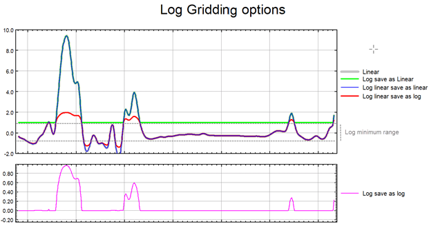
Log Options
If the data range is very wide and spans over several orders of magnitude, gridding in normal space may not honour the data distribution of interest, and the real patterns present in the data may get obscured in the process of gridding. If, however, the data is gridded in logarithmic space these very patterns will be revealed. Often it is more appropriate to grid geochemical data in logarithmic scale, as the element distribution changes in concentration by orders of magnitude over a short distance. Furthermore, depending on the data concentration and scatter, in order to maintain a consistent texture, it may be more appropriate to display the extremes of the data distribution in logarithmic space while the median range remains in linear space. This would be an appropriate approach with bimodal data.
Highly skewed data, such as geochemical data, can present a problem due to the disproportionate effect that high data values have on the surrounding region. For example, in a geochemical survey where the majority of chemical concentrations are in the range of not detectable to 100 ppm, the odd reading of many thousand ppm becomes weighted too strongly.
To overcome this effect, you can use the logopt parameter to take the log of the data before gridding. Once the data is gridded, you have the option of either restoring the original linear data scaling, or storing the logarithmic data in the output grid.
Logarithmic grids can be contoured by CONTOUR by selecting the logopt parameter in the CONTOUR control file. This option causes CONTOUR to expand any label numbers back to a linear scale before plotting the label. Note that the contour intervals must be selected logarithmically. The most typical logarithmic plot would use two contour levels, 0.25 and 1. Only the 0,1,2,3... levels would be labelled, and CONTOUR would label them 1,10,100,1000...
The log-linear options are not appropriate for geochemical data; they are intended for levelled geophysical data (e.g., sometimes the span of magnetic data is quite broad and in order to be able to observe the definition around the mean of the data distribution as well as at the extremes, this option is used). Prior to gridding the data for the two log-linear options, the data is altered as follows:
if ( Z > Log_minimum)) Z = (log10( Z / Log_minimum) + 1.0) * Log_minimum); if ( 0 < Z ≤ Log_minimum)) Z is untouched if ( -Log_minimum ≤ Z ≤ 0)) Z = -Z if ( Z < -Log_minimum)) Z = -(log10( -Z / Log_minimum) + 1.0) * Log_minimum); |
This has the effect of treating large positive or negative values like logarithms, but gives a linear transform for values around zero.
Log minimum value: when gridding in log space, this setting specifies the minimum cut-off in linear space. If one of the log, save as options has been selected, all values below this cut-off are replaced by Log_minimum. If one of the log-linear,save as options has been selected, this entry represents the two boundaries where the switch between linear and logarithmic gridding occurs.
The illustration below intends to convey the variation between the various log options.
Low-pass Desampling Factor
The de-sampling factor is defined as a function of the grid cell size. Before any further calculations, all points within cells of dimension cell_size x desampling_factor are averaged into a single value and placed in the center of the cell.
The default desampling (desampling_factor) is set relative to the contributing points as:

Desampling has two impacts:
Effectively it acts as a low-pass filter. The larger this parameter the smoother the output grid.
Speeds up the variogram calculation when the input database is very large.
If the database contains less than 100000 contributing points, the default is set to 1, and the only pre-filtering consists of de-aliasing at the cell level.
The variogram calculation duration is a function of the square of the contributing points. Increasing this factor visibly cuts down the variogram calculation time while little impact is seen on the variogram curve.
The Variogram File Format
The kriging method (KRIGRID) will write out the variogram of the data in the (*.var) file specified.
/ ------------------
/ MODEL = SPHERICAL
/ NUGGET = 0
/ RANGE =22098.416
/ SILL = 98.531197
/ SIGMA = 22.876097
/
/ VH VG VGM NP I
/ ---------------------------------------------------
0 0 0 691 0
642.3125 46.7532 4.294652 156 1
1149.407 56.01426 7.680435 1893 2
1917.167 62.67951 12.79007 2621 3
The file is a standard Geosoft data file (ASCII text) that begins with comment lines containing information about the variogram model, in this case a spherical model . The model parameters are listed (model, nugget, sill, and range), together with SIGMA, which is the RMS difference between the variogram model and the observed variogram. The data columns contain the distance between samples (VH), the observed variogram (VG), the modelled variogram (VM), the number of points averaged to calculate the variogram (NP), and an index (I).
Anisotropic Gridding
In many, if not most, geologic situations, there is a natural bias (anisotropy) of the features of interest in the direction of geologic strike. You can create a grid enhanced in a preferred direction using the strike direction and a weighting factor. This method enables you to incorporate the dominant geologic strike and define a preferential weighting in the strike direction, enhancing geological trends in your dataset. This effectively creates an "ellipse" with the major axis in the direction of strike, and the minor-axis perpendicular to the strike.
The Strike weight (>0.0) is the elliptical weighting (or preference) to apply along strike. The default value of 1.0 creates NO directional bias in the data. Typically, if your data is biased along strike, set the weighting to 2.0. This doubles the importance of data along strike. You can adjust the weighting to achieve a desired outcome by looking at results and experimenting a bit.
A second and related use of these parameters is to correct for anisotropy in the observed sampling pattern. Statistical kriging works best when data is nominally evenly distributed. If you have data collected on lines at a high sample density relative to line separation, you should set the strike direction to be perpendicular to the lines, set the strike weight to be the line separation divided by the along-line sample interval.
The Krigrid Log Report File
Kriging produces a log report of the gridding process. The report gives details about the input data and lists the Kriging parameters. The GX lists the calculated and model variogram, performs the kriging and reports each grid row as it is completed; and finally writes out the output grid and reports the grid parameters.
_______________________________________________________________________
Operating system version
Copyright Information
Gridding Start timestamp
Number of input contributing data points
Number of data points after clustering
KRIGRID Control Parameters:
Grid Cell Size
Grid Origin
Grid Size
Grid Dimensions
Is area clipped ?
Column to grid
Log option
Minimum value for log option
Desampling factor
Blanking Radius
Min/Max Search Radius
Min/Max Search points
Use octant search
Use all data points
Remove trend ?
Variogram model
Variogram power
Variogram model nugget
Variogram model slope
Max. Dist. of Variogram Analysis
Inc. Dist. of Variogram Analysis
Output Grid Specifications:
# points per record
# records
Variogram Analysis:
Model type
Nugget
Slope
Power
Sigma
Variogram_distance_bin Observed_Variogram_value_for_bin Model_Variogram_value_for_bin Number_of_points_in_Bin Bin_Number
.
.
.
Gridding end timestamp
_______________________________________________________________________
Got a question? Visit the Seequent forums or Seequent support
© 2023 Seequent, The Bentley Subsurface Company
Privacy | Terms of Use