Grid Data - Bi-directional

Gridding refers to the process of interpolating data onto an equally spaced “grid” of cells in a specified coordinate system. For an introduction to gridding and a summary of the different gridding methods click here.

Bi-directional Gridding

The bi-directional gridding method (BIGRID) rapidly interpolates roughly parallel line-based data. BIGRID uses linear, minimum curvature, or Akima splines to interpolate grid nodes between lines. The method is suitable for highly sampled data surveyed along regular lines (can work well with potential field geophysical data), and it is ideal for line-oriented data because it inherently tends to strengthen trends perpendicular to the direction of the survey lines. In this way, BIGRID can take advantage of the fundamental characteristics of line-based surveys. The method cannot be applied to randomly distributed XYZ data. Line data that is measured along orthogonal lines is also not well suited to BIGRID. For an overview of the method click here.

To perform bi-directional gridding, you must supply a data channel, an output grid name, and optionally the grid cell size. In addition, you have a variety of options, including the ability to:

• apply linear and non-linear filters to the original line data.

• The use of the non-linear filter is a very effective way to remove data spikes (undesired high-amplitude short-wavelength features) from the original data.

• grid the original data or its logarithmic representation.

• apply trend removal based on the orientation of geologic features.

• select a spline method (e.g., linear, cubic, Akima)

• define the grid coverage (spatial limits of the area to be gridded, cells to extend beyond data).

Use the Grid Data option from the Grid and Image > Gridding menu to grid data using the bi-directional gridding algorithm.

Bi-directional – Gridding Options

Data to grid	Select the database channel to grid. To specify an array element, append to the channel array name the element index in square brackets. For example, Chan[1] would indicate the second element of the array channel "Chan". Script Parameter: BIGRID.CHAN
Output grid	Provide the name of the output grid file. This field is auto populated based on the active database and the selected channel to grid; however, you can override the default. The default output grid format is selected automatically as the output file type. The type can be controlled using the browse dialog, which is accessible from the [...] button.  Script Parameter: BIGRID.GRID
Gridding method	The current gridding method is displayed. Script Parameter: GRIDDING_TOOL.METHOD [Bi-directional: 1]
Cell size	Specify a cell size for the output grid. The grid cell size is the distance between grid points in the X and Y directions. This field is auto-populated with the calculated default grid cell size and rounded to the nearest ten or hundred. Default grid cell size The default cell size is calculated as the greater of: 1/8 of the average line spacing (cross-line separation) the average of data sample spacing/station interval (along-line separation) See the Application Notes below for more details on adjusting the grid cell size. Script Parameter: BIGRID.CS
Extents and Data
Spatial Extents
Grid extents (X min, Y min, X max, Y max)	Define the spatial limits of the area to be gridded. By default, these fields are set to the full extents of the current X & Y channels of the active database in order to include all the data in the database: X min, Y min: the ground coordinates of the first grid point at the bottom left corner of the rectangular grid area (by default, the minimum limits of the input data file are used). X max, Y max: the ground coordinates of the last grid point at the top right corner of the rectangular grid area (by default, the maximum limits of the input data file are used). To grid a subset of the data, enter the limits of the bounding rectangle, or press the Draw Extents button to interactively define the boundary extents – the output grid coverage will extend to these limits. Script Parameter: BIGRID.XYRANGE
[Draw Extents]	Press this button to interactively define the grid boundary extents: in the Grid Preview pane, use the mouse to click & drag to draw a box, then release the mouse cursor to accept the final size of the box. The X & Y values will be updated in the Grid extents fields, and the preview window will be refreshed to show the newly defined extents. You can draw the box in any of the four possible ways (e.g., from bottom left to top right).
[Reset Extents]	Press this button to reset the grid extents to the initial state of defaults for the active database. The Grid Preview pane (when Auto-refresh is enabled) will be updated to reflect the change; however, the zoomed state (in/out) of the grid preview will not be affected.
Max line separation	Enter the maximum separation distance, in data units, allowed between lines. Areas enclosed by lines that are farther apart than this distance are represented by dummy values in the output grid. By default, the maximum separation is set to 1.7 times the maximum line separation. If the line to line separation maximum is too narrow, the output grid will consist of data strips that frame each survey lines with blank grid areas in between. The width of the data strips will depend on the number of cells that extend beyond the edges of the data in line 2 of the control file. Script Parameter: BIGRID.SMX
Max point separation	Enter the maximum separation distance, in data units, allowed between stations. Gaps in lines wider than the station to station maximum are not interpolated. By default, the maximum separation is set to zero, which indicates that all values are interpolated. If the entered value is smaller than the output cell size, then internally it is increased to be equal to the output cell size. Script Parameter: BIGRID.GAPLIM
Cells to extend beyond data	The number of cells to extend beyond the edges of the data. By default, the number of cells is set to 1 when gridding data, which ensures that the grid will always extend at least a fraction of a cell past the ends of valid data. When re-gridding grids, the number of cells is set to 0 by default to prevent growth of the grid. Setting the number of cells beyond the edges of the data to 2 or 3 and the maximum separation permitted between lines to the grid cell size will produce a strip grid. A strip grid will only have valid data in strips that frame the survey lines. This is an effective presentation when lines are too far apart to be gridded properly. Script Parameter: BIGRID.NEX
Data Filtering
Mask channel	Select a channel from the drop-down list to act as a mask. Only database channels that have the class property set as "MASK" are listed. Additionally, string channels and channels with array size greater than 1 are omitted from the list. The data values in the selected Data to grid channel with corresponding dummy (*) values in the Mask channel will not be used in the gridding process. The X & Y values will be updated in the Grid extents fields to reflect the masked data, and the generated masked grid (with the correct extents) will be automatically rendered in the Grid Preview window (the Auto-refresh option must be selected).  Script Parameter: BIGRID.MASK_CHANNEL
Log option	You can either grid the original data or its logarithmic (base 10) representation. Gridding the log of the data can be a very effective way to reduce distortion due to highly skewed data such as geochemical data. The options are: linear: grid the data as it is. log, save as linear: grid the data in logarithmic space and clip all values less than ‘Log minimum’ to the ‘Log minimum’ value, then convert the data back to linear space before saving it to the grid file. log-linear, save as linear: grid the data above the positive ‘Log minimum’ and below the negative ‘Log minimum’ in logarithmic space (flip the sign of the data originally in the negative range to take the logarithm then inherit back the sign of the original data; grid the conditioned data). After gridding, all cell values outside the ± ‘Log minimum’ range are converted back to linear space and scaled to maintain continuity at the boundary. Data within the ± ‘Log minimum’ range remains intact and is gridded in a linear sense. Finally, the linear representation of the data (in both ranges) is saved to the grid file. log, save as log: same as ‘log, save as linear’ except that the grid values are kept in log space: the gridded values are saved to the grid file in their logarithmic representation. log-linear, save as log: same as ‘log-linear, save as linear’ except that the grid values are not converted back from log space. The output grid is in logarithmic space with the large amplitude anomalies being somewhat moderated. See the Application Notes below for more details. Script Parameter: BIGRID.LOGOPT   linear: 0   log, save as linear: -1   log-linear, save as linear: -2   log, save as log: 1   log-linear, save as log: 2
Log minimum value	If gridding in log space (see the Log options above), this parameter specifies the minimum value. The default is 1. See the Application Notes below for more details. Script Parameter: BIGRID.LOGMIN
Interpolation
Bi-directional
Low-pass filter wavelength	Specify the low-pass filter wavelength. To apply a low-pass filter, specify only the short wavelength cut-off. The low-pass cut-off is specified in the same distance units as the data file. See the Application Notes below for more details on BIGRID filters. Script Parameter: BIGRID.WS
High-pass filter wavelength	Specify the high-pass filter wavelength. To apply a high-pass filter, specify only the long wavelength cut-off. The high-pass cut-off is specified in the same distance units as the data file. See the Application Notes below for more details on BIGRID filters. Script Parameter: BIGRID.WL
Non-linear filter tolerance	Specify the tolerance in "Z" units (e.g. gammas) for the non-linear filter. Non-linear filtering uses logic to determine if a given data point is part of the short wavelength information to be removed or not. The decision is based first on wavelength, then on an amplitude tolerance. If based on wavelength, a data point is considered part of the short wavelength information. It’s amplitude, relative to a local background, is compared to the non-linear filter tolerance. If it exceeds this tolerance, it is removed from processing and replaced by a local background value. If the non-linear filter tolerance is blank, the non-linear filter is not applied. See the Application Notes below for more details on BIGRID filters. The non-linear filter is excellent for removing data spikes. The cut-off wavelength used for the non-linear filter is the same as the wavelength specified for the low-pass filter (see the above section). Script Parameter: BIGRID.TOLN
Pre-filter sample increment	Specify a pre-filter sample increment. If the distance between each data point on a line differs by more than the default tolerance (2%), the line is first re-sampled at an increment using the down-line spline. The data is then filtered and splined again to the grid cell size. By default, the resample increment is set to the smaller of the grid cell size or the smallest data increment on the first survey line. Script Parameter: BIGRID.FDX
Data pre-sort option	Select from one of the options available: "none", "pre-sort data", "remove backtracks". The default is "none". Presorting of the data will sort each line so that all data points are consecutive in the gridding direction. Caution should be exercised when presorting, because data entry errors may result in the data being sorted out of order. The "remove backtracks" option will cause data in the line that appears to backtrack to be removed. Use this option when processing airborne geophysical data. Script Parameters: BIGRID.PRESORT
Spline down line	Geological trends in the data can be emphasized by the appropriate orientation of the grid so that the second interpolation is in the direction of strike. In addition to trend enhancement, BIGRID allows the method of interpolation to be selected independently for the down-line and across-line directions. Select from one of the interpolation methods available: linear, cubic spline (minimum curvature), Akima spline (default), or "Nearest neighbour". For data that is sampled at a high density relative to the grid cell size, such as is often the case for airborne data, linear interpolation is usually sufficient for the down-line spline and will produce some saving in computation time. Script Parameter: BIGRID.ISP1
Spline across line	Select the across-line interpolation method as "Cubic", "Akima", "Linear" or "Nearest neighbour". The default is "Akima". In cases where the data contains rapid changes in gradient, the minimum curvature (cubic) spline may produce undesirable highs or lows in the final grid. This most commonly occurs across lines with poor line-to-line correlation of the data. The Akima spline method does not suffer as much from this problem, although it does tend to produce sharper corners around actual data points and the resulting grid tends to be less smooth. Script Parameter: BIGRID.ISP2
Trend angle	Specify the trend angle measured counter-clockwise relative to the positive X-axis (deg ccw from +X).This parameter is intended to enhance geological features in the direction specified. If the trend angle is not specified, the default is to calculate the angle perpendicular to the survey line direction. See the Application Notes for more details on specifying the trend angle. Script Parameters: BIGRID.TRA
Force grid direction	Select the grid direction as "default", "for vertical lines (KX = 1)", or "for horizontal lines (KX = -1). If the survey lines run in the Y direction (vertical), KX should be 1; if the survey lines run in the X direction (horizontal), KX should be -1. By default, BIGRID will choose KX so that the second interpolation direction is closest to perpendicular to the average line direction (i.e. the average of all lines) unless a trend angle is specified, in which case KX will be 1. The output grid direction parameter (represented by KX) determines whether the output grid lines will be parallel to the output grid X-axis (KX = 1) or the Y-axis (KX = -1). The variable KX should be chosen such that: the first interpolation is close to the survey line direction or, the second interpolation, which defines the direction of the output grid lines, is across the survey lines. Script Parameters: BIGRID.KX
Use gradient enhanced gridding*	Check this option if you have horizontal gradient data that you would like to use in the gridding process. This will enable the Gradient Enhancement tab. Refer to the Application Notes below for additional information on gridding with gradient data. When data along the survey line is adequately sampled, splining along the survey direction honours the observed data. However, splining across the survey lines has more freedom to deviate from the true ground response. Supplying this gradient restricts the freedom in the direction normal to the primary survey direction and improves on the conformity of the splined data with the actual ground response.
Gradient
Gradient Enhancement*
Transverse gradient data	Select the data channel that contains the transverse gradient data. The gradient should be expressed in data units/units of distance measurement in your X,Y coordinate system. For example, gradient magnetic data in a UTM coordinate system must be in units of nT/m. Refer to the Application Notes below for additional information on gridding with gradient data. Script Parameter: BIGRID.GRAD
Gradient sensor separation	You can optionally specify an apparent sensor separation (in the same units as the XY data) that will be used to reconstruct original data from the gradient information. In the case of an airborne magnetometer survey, this would be the wing-tip separation if the sensors are located in the tip of each wing. If the data is not well levelled, a wide sensor separation may introduce noise, counteracting the gradient gridding. In this eventuality, it is recommended to decrease the sensor separation to a fraction of the cell size. If not specified, a separation of 1/20 the grid cell size is used. Script Parameter: BIGRID.GSEP
Gradient direction	Select the gradient direction as "parallel to line (forward)" or "perpendicular to line (right)". This option controls if the gradient data will be corrected for line direction. If you have preprocessed and leveled your gradient data yourself, or if it has been prepared by a survey contractor, it is likely already oriented to be "parallel to line (forward)". You can check this by plotting the gradient profiles on a flight plan map. You may also have gradient data that is simply the difference between the right and left sensors, in which case the gradient will be "perpendicular to line (right)". In this case, the gradient will be corrected for the line direction to be in the gridding direction. The direction of each line is determined from the first and last point in each line, and the along-line gradient is used to calculate the correct gradient in the gridding direction indicated by the trend angle parameter. Script Parameter: BIGRID.GCOR [0 – parallel, 1 - perpendicular]
Correct gradient levels	If your gradient data contains "heading" error, you may choose to correct each line by leveling the mean of the measured gradient data to match the gradient calculated from the total field data. If the gradient data is already sufficiently well corrected and compensated, correcting the gradient levels can actually introduce noise because of the possible inaccuracy of the average calculated gradient background levels. This can be more of a problem with relatively short lines. Script Parameter: BIGRID.GLEV
Gradient noise level	Specify the nominal gradient noise level to be used to blend more accurately the calculated gradient. Raw measured gradient data can have quite poor resolution at very long wavelengths, which tend to have very low absolute gradients. This can introduce noise in the smooth parts of a survey area. If you specify the noise level of your gradient data, the gradient calculated from the total field will be blended together with the measured gradient to minimise this problem. Click to expand the "blending" algorithm.  G = (Gg + Gm * SN) / (1 + SN)  SN = abs(Gm/N) Where:  G: the merged gradient to use in gradient gridding.  Gg: the gradient calculated from gridded total field.  Gm: the measured gradient.  SN: the signal to noise ratio at each point  N: the measured gradient noise level Script Parameter: BIGRID.GNOISE
[Restore Defaults]	This button remains disabled until any of the fields default values are changed. Press the button to reset the gridding parameters to the initial state of defaults for the active database. When Restore Defaults is clicked: The following parameters are reset to their default values: The cell size value All the parameters on both the Extents and Data and Interpolation tabs Only the parameters for the current gridding method are affected. The following parameters are not reset: The data to grid selection The output grid file name The gridding method The Grid Preview (with Auto-refresh enabled) and Variogram panes will be updated to reflect any parameters changes; however, the zoomed state (in/out) of the grid preview will not be affected.

Application Notes

BIGRID generates a grid file (*.GRD) using a two-step process:

1. Each line is interpolated along the original survey line to yield data values at the intersection of each required grid line with the observed value.

2. The intersected points from each line are then interpolated in the across-line direction to produce a value at each required grid point.

The second pass of interpolation creates the grid lines. A grid line is a series of numbers that represent all the values along a single grid row.

Adjusting the Cell Size

As this gridding method might not always be able to determine an accurate line and sample separation, we recommend that you always review the grid cell size of the output grid and change it if necessary. In practice, the grid cell size should not be smaller than ⅛ the nominal line separation. If the cell size is unreasonably small, short-wavelength linear features that trend perpendicular to the survey lines can be introduced into the grid, especially if the input data is noisy.

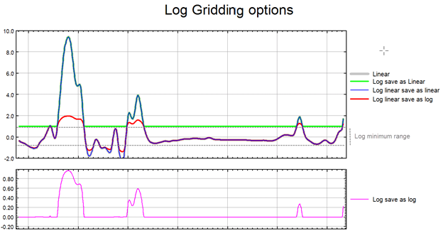
Log Options

The log-linear options are not appropriate for geochemical data; they are intended for levelled geophysical data (e.g., sometimes the span of magnetic data is quite broad and in order to be able to observe the definition around the mean of the data distribution as well as at the extremes, this option is used).

Prior to gridding the data for the two log-linear options, the data is altered as follows:

if ( Z > Log_minimum))  Z = (log10( Z / Log_minimum) + 1.0) * Log_minimum);

if ( 0 < Z ≤ Log_minimum))  Z is untouched

if ( -Log_minimum ≤ Z ≤ 0))  Z = -Z

if ( Z < -Log_minimum))  Z = -(log10( -Z / Log_minimum) + 1.0) * Log_minimum);

This has the effect of treating large positive or negative values like logarithms, but gives a linear transform for values around zero.

Log minimum value: when gridding in log space, this setting specifies the minimum cut-off in linear space. If one of the log, save as options has been selected, all values below this cut-off are replaced by Log_minimum. If one of the log-linear,save as options has been selected, this entry represents the two boundaries where the switch between linear and logarithmic gridding occurs.

The illustration below intends to convey the variation between the various log options.

Optimizing Bi-Directional Line Gridding with Oblique Survey Lines

The trend angle is intended to enhance geological features in the direction specified. Since ideally you want to enhance features perpendicular to the survey line direction, you should specify this angle to be perpendicular to the line direction. Note that the angle to be specified is counter-clockwise relative to the positive X-axis (which normally points to the east).

If the line direction is very close to either north-south or east-west, BIGRID’s default settings are ideal. If the survey lines are at other angles (not in the north-south or east-west orientations), you should override the default BIGRID settings to avoid odd streaking or other non-geological results. For example, if your survey lines are oriented at N30E, specify a trend angle of either –30 degrees or 150 degrees. If your survey lines are oriented at N45W, specify a trend angle of 45 degrees. This approach will also enhance geological trends perpendicular to the line direction.

Gradient Enhanced Gridding

Gridding without the cross-line gradient will interpolate the smoothest surface that honors the data along each line. Gridding with the cross-line gradient will produce a surface that both honors the data and the measured gradient at each line. This can produce much-improved gridded surfaces, especially for features that approach the line separation in size.

Gridded magnetic data: a) without cross-line gradient; b) with cross-line gradient enhancement.

The gradient-enhanced method implemented in BIGRID is the pseudo-line gridding method developed by Hardwick ¹.

Although gridding with gradients will work with any type of data, the principle application is in the preparation of grids from aeromagnetic surveys that use two wing-tip sensors to measure the transverse gradient. The technique used in BIGRID uses both the measured total field data and the gradients to model the magnetic field over the grid area. This requires that both the total field and the gradient data be well leveled using conventional leveling techniques. This method also ensures accurate resolution of low-amplitude, long-wavelength features in the data, which are poorly resolved in the gradient measurements alone.

Following are potential sources of error when working with gradient dataL

1. Aircraft orientation error. Because of the orientation of the survey aircraft in flight, gradients may not be measured on a true horizontal plane. However, provided the survey is conducted to minimize aircraft maneuver, this noise is normally minimal.

2. Aircraft control surface error. The simple movement of the aircraft control surfaces – notably the ailerons, can introduce magnetic noise to wing-tip sensors. Surveys should be flown with this in mind, and survey pilots should be more concerned with minimizing the use of ailerons over attempting to maintain a very accurate flight path and elevation. Low-pass filters can be used to remove aileron noise if necessary, though this noise often overlaps signal of interest, so such data will be degraded.

3. Actual horizontal gradients can be very small, often less than the noise level in the measured gradient. If long-wavelength, low-amplitude features are of interest, you should specify the noise level of the gradient data so that this information can be accurately recovered from the total field data.

4. Gradient data that is not properly compensated for aircraft orientation, notably for heading error, can contain base level differences that vary relative to the line direction. In this case, the measured gradient data can be corrected so that the mean matches the mean of the calculated gradient along each line. This should only be done if the data has not been properly compensated as this technique may introduce noise where the calculated gradient is inaccurate.

BIGRID Filters

One of BIGRID's most powerful features is its ability to design and apply non-linear and/or linear numerical filters to the original line data before interpolation. The use of the non-linear filter is a very effective way to remove data spikes (undesired high-amplitude short-wavelength features) from the original data.

It is a good idea to apply filters routinely to remove frequencies higher than the Nyquist frequency of the output grid (1 / (2*grid cell size)) or, equivalently, wavelengths shorter than twice the sampling interval (2*grid cell size). This is important to insure that aliasing of higher frequency signal does not occur in the final grid. See Reid ¹ for a brief discussion of aliasing and its effect on survey design.

The filter wavelengths can also be set to whatever values would be appropriate for the data at hand.

The filters require evenly spaced data down each line. If this is not the case, the data must be re-sampled (before the filters are applied) by specifying (in the control file) a sample interval (FDX) set to the minimum station interval.

The filters are applied in two optional steps. If a non-linear filter is requested, it is the first filter applied. The linear filter is then applied. To apply the filters, BIGRID will extend the data at the ends of each data line to account for the width of the numerical operations. The extended points are calculated using Burg's ² maximum entropy method that insures that the extended parts of the line have the same spectral characteristics as the original data.

The Non-Linear Filter

The non-linear filter after Naudy and Dreyer³ is a low-pass filter that removes signal based on logic and has two important advantages over linear filtering alone:

1. It ignores signal power and can therefore cleanly remove very strong signal without the familiar long-wavelength residual left by linear filters.

2. When data does not contain signal to be removed it is not changed at all and therefore contains all the original information.

The short wavelength cut-off point of the non-linear filter is the value specified by the parameter (WS) in the BIGRID control file.

Any signal determined to be within the noise level by the non-linear operator, but that has amplitude smaller than the specified tolerance (TOLN), is not altered by the filter. The default tolerance of approximately 1% of the maximum amplitude of the input data set should be sufficient for almost all cases. By setting a larger tolerance, low amplitude real signal may be protected from filtering when attempting to remove much higher amplitude noise. Think of the tolerance as an envelope surrounding the data within which the data is not altered regardless of wavelength.

The Linear Filter

After applying the non-linear filter, a linear filter after Fraser and others⁴, is designed and applied to the data along survey lines.

The short wavelength cut-off point for the linear filter is half the wavelength (WS) specified for the non-linear filter. If this is greater than twice the sampling interval, the sampling interval is used. The half short wavelength cut-off limit is used because the only purpose of the low-pass part of the linear filter is to smooth any remaining point-to-point chatter that may remain after non-linear filtering.

The number of coefficients in the filter is taken as twice the length of the longest wavelength to be left in the data (up to a maximum length of 512 coefficients). If a low-pass filter is being applied, as it is usually the case, only the short wavelength cut-off point is used to calculate the optimum filter length.

BIGRID only filters down actual survey lines. The resulting grid is not filtered across the survey lines in the trend direction. To do this, the output grid can be re-gridded with the same filter specifications so that across line filtering is applied. This works because the output grid lines are always perpendicular to the input survey lines and the program filters grid lines when re-gridding grids.
This re-gridding would only be necessary in special cases when band-pass filtering or long wavelength low-pass filtering is being performed. After the second pass of BIGRID there may be some high-frequency grid-line to grid-line signal left in the data. This can be removed by applying a 2-D Hanning filter, using GRIDHANN from the Geosoft grid utilities, until the desired grid result is achieved.

References

The Bigrid Log Report File

The "bigrid.log" file is produced with each run and contains information about the bi-directional gridding process, including lines skipped due to backtracks or clipping.

The Bigrid CON  File

BIGRID creates a control file in your project folder. This file ("_bigrid.con") is then used by the gridding process. You can also build a BIGRID control file through a text editor and take advantage of further specialized settings not available through the Grid Data. To learn more, go to topic Bi-directional Griding from a Control File.

Reference

References

- [1] A. B. Reid, "Aeromagnetic survey design", Geophysics, vol. 45, no. 5 (1980), pp. 973-976 .
- [2] J. P. Burg, "Maximum entropy spectral analysis", Ph.D. Thesis, Dept. of Geophys., Stanford Univ., 1975.
- [3] H. Naudy and H. Dreyer, "Essai de filtrage non-lineaire appliqué aux profils aéromagnétiques (Attempt to apply nonlinear filtering to aeromagnetic profiles)", Geophysical Prospecting, vol. 16, no. 2 (1968), pp. 171-178 .
- [4] D. C. Fraser, B. D. Fuller, and S. H. Ward, "Some numerical techniques for application in mining exploration", Geophysics, vol. 31, no. 6 (1966), pp. 1066-1077
DOI: https://doi.org/10.1190/1.1439840