
Grid Data - Minimum Curvature
Gridding refers to the process of interpolating data onto an equally spaced “grid” of cells in a specified coordinate system. For an introduction to gridding and a summary of the different gridding methods click here.
Minimum Curvature Gridding
The minimum curvature gridding method fits a minimum curvature surface, which is the smoothest possible surface that will fit the given data values. The method is suitable for data with a relatively large number of samples (it can work well with geochemical data from comprehensive regional and local surveys), and it is best used when data is randomly distributed, sampled along arbitrary lines, or if you want to include tie lines. For an overview of the method click here.
To perform minimum curvature gridding, you must supply a data channel, an output grid name, and optionally the grid cell size. In addition, you have a variety of options, including the ability to:
-
define the grid coverage (spatial limits of the area to be gridded, cells to extend beyond data).
-
grid the original data or its logarithmic representation (using cutoffs or a data range).
-
grid your data in a more compact and efficient way by gridding parallel to survey lines
-
specify desampling values (for low-pass filtering) and a blanking distance (for removing values beyond a certain distance).
-
define the tolerance to which the minimum curvature surface must match the data points and the percentage of points that must meet the tolerance for the iterations for the current processing step to stop.
-
specify the maximum number of iterations to allow.
-
adjust the tension to produce a true minimum curvature grid or to increase the tension to reduce overshooting problems in unconstrained, sparse areas.
The gridding process generates a grid file (*.grd) and a gridding report file (rangrid.log). The report file gives details about the input data and the parameters that were used for processing.
Use the Grid Data option from the Grid and Image > Gridding menu to grid data using the minimum curvature gridding algorithm.
UXO-Marine extension:
- UXO-Marine Sonar Utilities menu
Minimum Curvature – Gridding Options
|
Data to grid |
Select the database channel to grid. To specify an array element, append to the channel array name the element index in square brackets. For example, Chan[1] would indicate the second element of the array channel "Chan". Script Parameter: RANGRID.CHAN |
|
Output grid |
Provide the name of the output grid file. This field is auto populated based on the active database and the selected channel to grid; however, you can override the default. The default output grid format is selected automatically as the output file type. The type can be controlled using the browse dialog, which is accessible from the [...] button. Script Parameter: RANGRID.GRID |
|
Gridding method |
The current gridding method is displayed. Script Parameter: GRIDDING_TOOL.METHOD [Minimum curvature: 0] |
|
Cell size |
Specify a cell size for the output grid. This field is auto populated with the calculated default grid cell size and rounded to the nearest ten or hundred: The grid cell size (the distance between grid points in the X and Y directions) should normally be ¼ to ½ of the line separation or the nominal data sample interval. If not specified, the data points are assumed to be evenly distributed, and the area rectangular. The default cell size is then defined by the following formula:
Where:
See the Application Notes below for more details on adjusting the grid cell size. Script Parameter: RANGRID.CS |
Extents and Data |
|
Spatial Extents |
|
|
Grid extents |
Define the spatial limits of the area to be gridded. By default, these fields are set to the full extents of the current X & Y channels of the active database in order to include all the data in the database:
To grid a subset of the data, enter the limits of the bounding rectangle, or press the Draw Extents button to interactively define the boundary extents – the output grid coverage will extend to these limits. Script Parameter: RANGRID.XY |
|
[Draw Extents] |
Press this button to interactively define the grid boundary extents: in the Grid Preview pane, use the mouse to click & drag to draw a box, then release the mouse cursor to accept the final size of the box. The X & Y values will be updated in the Grid extents fields, and the preview window will be refreshed to show the newly defined extents. |
|
[Reset Extents] |
Press this button to reset the grid extents to the initial state of defaults for the active database.
The Grid Preview pane (with Auto-refresh enabled) will be updated to reflect the change; however, the zoomed state (in/out) of the grid preview will not be affected.
|
|
Blanking distance |
Specify the blanking distance: grid cells farther than this value from a valid point will be set to dummies in the output grid. Preferably, this parameter should be set to just greater than the maximum distance through which interpolation is desired. Normally, the blanking distance and the grid cell size should be set in conjunction. If no value is entered for the blanking distance, then the grid will cover the maximum limits of the data plus eight times the grid cell size. If a grid node is closer to at least one observed data point than the blanking distance, it will be calculated, and otherwise it will remain blank. This field is auto populated with the calculated default value as per following formula:
Where:
Script Parameter: RANGRID.BKD |
|
Cells to extend beyond data |
This is the number of grid cells to extend beyond the outside limits of the data. The default is the integer value of blanking distance/grid cell size. If the X and Y range values are not defined, the grid size will be set to the actual data range plus this value. This parameter is commonly used in conjunction with the blanking distance parameter. For best results, use the blanking distance parameter to control the amount of coverage around data and this parameter to set the default grid size – with this distance generally being smaller than the blanking distance to provide clipping around the grid. Script Parameter: RANGRID.EDGCLP |
Data Filtering |
|
|
Mask channel |
Select a channel from the drop-down list to act as a mask. Only database channels that have the class property set as "MASK" are listed. Additionally, string channels and channels with array size greater than 1 are omitted from the list. The data values in the selected Data to grid channel with corresponding dummy (*) values in the Mask channel will not be used in the gridding process. The X & Y values will be updated in the Grid extents fields to reflect the masked data, and the generated masked grid (with the correct extents) will be automatically rendered in the Grid Preview window (the Auto-refresh option must be selected). Script Parameter: RANGRID.MASK_CHANNEL |
|
Log option |
You can either grid the original data or its logarithmic (base 10) representation. Gridding the log of the data can be a very effective way to reduce distortion due to highly skewed data such as geochemical data. The options are:
See the Application Notes below for more details. Script Parameter: RANGRID.LOGOPT |
|
Log minimum value |
If gridding in log space (see the Log options above), this parameter specifies the minimum value. The default is 1. See the Application Notes below for more details. Script Parameter: RANGRID.LOGMIN |
Interpolation |
|
Minimum Curvature |
|
|
Low-pass desampling factor |
Specify the desampling factor as a multiple of the grid cell size. This effectively acts as a low-pass (smoothing) filter by averaging all points into the nearest cell defined by this factor. Leaving the default value (1) results in no pre-filtering other than de-aliasing by averaging data points within a cell. Script Parameter: RANGRID.DSF |
|
Starting coarse grid |
Select a value from the available options (16, 8, 4, 2, 1) to indicate the desired coarseness of the starting iteration level relative to the final grid cell size. The default is 16, which is suitable for most datasets. Reducing this value will increase the processing time and resolve the densely sampled areas more accurately. See the Application Notes below for further details. Script Parameter: RANGRID.ICGR |
|
Search radius |
The maximum search radius in number of cells to use for establishing the starting grid values for the coarse grid. For any grid node, if no data points are found within this radius, the mean value of the observed data is used as the starting value. The default is defined as:
See the Application Notes below for more details. Script Parameter: RANGRID.SRD |
|
Weighting power |
The weighting power is used to generate the coarse starting grid. Values within a coarse cell are weighed by the inverse of their distance from the coarse grid nodes raised to this power. See the Application Notes below for more details on weighting power and the overall weighting formula. Script Parameter: RANGRID.IWT |
|
Weighting slope |
The weighting can further be moderated through the use of a slope parameter. The default value is 0.0, which means that the weighting formula is not applied, and only the data point nearest to a grid node is assigned to the node. If weighting slope is set to a value greater than zero, all data points within a block grid unit at each refinement level are weighted and used. See the Application Notes below for more details on weighting slope and the overall weighting formula. Script Parameter: RANGRID.WTSLP |
|
Tolerance |
The maximum permissible deviation of the fitted minimum curvature value from the initial value assigned to the node. Specify the tolerance required for each grid cell (absolute error, in grid data units). The default is 0.1% of the maximum range of the observed data. See the Application Notes below for further details. Script Parameter: RANGRID.TOL |
|
% Pass tolerance |
The required percentage of points that must pass the tolerance. The default is 99%. For a more accurate grid, increase the percentage. Script Parameter: RANGRID.PASTOL |
|
Max iterations |
The maximum number of iterations at each level of grid refinement after which the gridding algorithm does not proceed further. The default is 100. Basically, the gridding process stops if one of the following conditions is met:
See the Application Notes below for further details. Script Parameter: RANGRID.ITRMAX |
|
Internal tension |
The degree of internal tension (between 0 and 1). The default is no tension (0), which produces a true minimum curvature grid. Increasing tension can be used to prevent overshooting of valid data in sparse areas; however, curvature in the vicinity of real data will increase. In general, the more sparse areas are present in the data (with localized highs and lows), the higher the tension should be set. See the Application Notes below for more details on applying internal tension. Script Parameter: RANGRID.TENS |
|
|
|
|
[Restore Defaults] |
This button remains disabled until any of the fields default values are changed. Press the button to reset the gridding parameters to the initial state of defaults for the active database. When Restore Defaults is clicked: The following parameters are reset to their default values:
The following parameters are not reset:
The Grid Preview (with Auto-refresh enabled) and Variogram panes will be updated to reflect any parameters changes; however, the zoomed state (in/out) of the grid preview will not be affected. |


Application Notes
Once a gridding task is executed, the gridding options are retained when switching between different databases. The Grid Data tool will recall the previous gridding parameters associated with the current database, regardless of whether gridding tasks have been performed on different databases since.
The minimum curvature gridding creates a control file in your project folder. This file ( _rangrid.con) is then used by the gridding process. You can also build a RANGRID control file through a text editor and take advantage of further specialized settings not available through the Grid Data. To learn more, go to topic Minimum Curvature Gridding from a Control File.
Adjusting the Cell Size
Grid cell size should not be much less than half the nominal data point interval found in the areas of interest. A smaller cell size will more accurately fit the data points, but if the data contain errors this may not be desirable; it also means longer processing time and a larger output data size. A small cell size may also require a reduction in the iteration tolerance and an increase in the number of iterations to achieve an acceptable result. If the cell size chosen is smaller than the average data point density, then there will be many gaps in the output grid.
If the data is to be contoured (we recommend 2 mm or 1/10 inch at plot scale for contouring), specify a smaller cell size and a larger desampling factor or regrid the grid using bi-directional gridding.
With a larger cell size, the gridding algorithm averages more data points per grid node, thus the data appears smoother. However, increasing the cell size further is likely to introduce adverse results. It may dilute grid patterns that correspond to real geological features, thus obscuring real features. While dealing with large datasets, be aware of the trade-off between the processing accuracy and processing time, as well as the data storage requirements.
The choice of the grid cell should also be reflective of the intent of the gridding process. If the near-surface information such as in UXO investigation is of primary concern, the grid cell should be selected in the order of ~0.1 m. If the surface geological structure is of primary concern, such as in gold exploration, a larger grid cell should be selected – in the order of ~10m. If the deep seated geology is being investigated, such as in the case of oil exploration, the cell size can be much larger, in the order of ~100 m. A simple rule of thumb is to select the cell size roughly equal to the shallowest depth of interest.
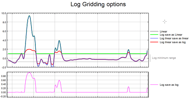
Log Options
If the data range is very wide and spans over several orders of magnitude, gridding in normal space may not honour the data distribution of interest, and the real patterns present in the data may get obscured in the process of gridding. If, however, the data is gridded in logarithmic space these very patterns will be revealed. Often it is more appropriate to grid geochemical data in logarithmic scale, as the element distribution changes in concentration by orders of magnitude over a short distance. Furthermore, depending on the data concentration and scatter, in order to maintain a consistent texture, it may be more appropriate to display the extremes of the data distribution in logarithmic space while the median range remains in linear space. This would be an appropriate approach with bimodal data.
Highly skewed data, such as geochemical data, can present a problem due to the disproportionate effect that high data values have on the surrounding region. For example, in a geochemical survey where the majority of chemical concentrations are in the range of not detectable to 100 ppm, the odd reading of many thousand ppm becomes weighted too strongly.
To overcome this effect, you can use the logopt parameter to take the log of the data before gridding. Once the data is gridded, you have the option of either restoring the original linear data scaling, or storing the logarithmic data in the output grid.
Logarithmic grids can be contoured by CONTOUR by selecting the logopt parameter in the CONTOUR control file. This option causes CONTOUR to expand any label numbers back to a linear scale before plotting the label. Note that the contour intervals must be selected logarithmically. The most typical logarithmic plot would use two contour levels, 0.25 and 1. Only the 0,1,2,3... levels would be labelled, and CONTOUR would label them 1,10,100,1000...
The log-linear options are not appropriate for geochemical data; they are intended for levelled geophysical data (e.g., sometimes the span of magnetic data is quite broad and in order to be able to observe the definition around the mean of the data distribution as well as at the extremes, this option is used). Prior to gridding the data for the two log-linear options, the data is altered as follows:
if ( Z > Log_minimum)) Z = (log10( Z / Log_minimum) + 1.0) * Log_minimum); if ( 0 < Z ≤ Log_minimum)) Z is untouched if ( -Log_minimum ≤ Z ≤ 0)) Z = -Z if ( Z < -Log_minimum)) Z = -(log10( -Z / Log_minimum) + 1.0) * Log_minimum); |
This has the effect of treating large positive or negative values like logarithms, but gives a linear transform for values around zero.
Log minimum value: when gridding in log space, this setting specifies the minimum cut-off in linear space. If one of the log, save as options has been selected, all values below this cut-off are replaced by Log_minimum. If one of the log-linear, save as options has been selected, this entry represents the two boundaries where the switch between linear and logarithmic gridding occurs.
The illustration below intends to convey the variation between the various log options.
Low-pass Desampling Factor
The data sampling density used when calculating a grid is controlled by the grid cell size. Highly sampled areas would have the tendency to manifest a higher noise level compared to the surrounding lower sampled regions. In some instances, you might want to further smooth the regions with a high level of clustering without affecting the more sparse regions. Low-pass desampling is an appropriate approach for smoothing this data and it effectively acts as a low-pass (smoothing) filter by averaging all points into the nearest cell defined by this factor. For example, a factor of 3 would first average database points into a coarse grid with cells size 3 times the final cell size.
The low-pass desampling factor parameter defines the size of the square within which the observed data is averaged. The data is subdivided into adjacent bins of this size within which at most one averaged value is retained. This value should be specified in terms of number of grid cells as opposed to distance units.
The parameter is generally used in conjunction with the Weighting power and Weighting slope parameters. The weighting power attributed to each observed data point is either the inverse distance to the grid node or the inverse distance squared. Furthermore, in order to counteract the aliasing problem, the weight slope factor can be used. Airborne data by nature has a high sampling rate along the traverse and low sampling rate across traverses. The weighting slope offers a means of moderating the distance weight factor, where the sharpness of the 1/dn (inverse distance or inverse distance squared) factor is moderated. For anisotropic data, such as airborne data, this factor provides a higher weight for lateral points, away from the traverse lines.
Data Point Weighting Settings
Two settings define how the gridded parameter values are weighted to produce the initial node values:
When generating the initial coarse grid, in order to come up with initial grid node values for grid cells that do not contain any observed data, grid node values beyond the grid cell are averaged using the weighting power setting. The weights are defined as:

Where:
D: distance between the grid node and grid cell points residing within the search radius but beyond the grid cell.
p: power applied to the distance.
The weighting slope is not used at this initial stage.
As the algorithm moves from the initial coarse grid to the refined grid, weighting can further be moderated through the use of a slope parameter, and both the weighting power and the weighting slope are used in the weighting formula:

Where:
D: distance between the contributing data point and the grid node given in fractions of the grid cell size.
p: power applied to the distance.
S: slope in cell units.
If the weighting slope is set to zero, neither weighting power nor weighting slope are used after the initial coarse grid has been processed. No weighting is performed on subsequent refined grid iterations, and only the data point nearest to a grid node affects the parameter value assigned to that node.
If the data has been collected along traverse lines, it is recommended to set the slope (S) as the number of grid points between the traverse lines.
The greater the value of the weighting slope setting, the more the weighting falls off according to the weighting power alone. Setting the weighting slope to a value greater than 0 is suitable for anisotropic datasets. For instance, in aeromagnetic survey data with a line spacing of 200 metres and readings every 5 metres along the line, the 50 metre cell size block will include a large number of real data points to be combined into one weighted location and z value; in such case, setting the weighting slope to 5.0 will produce a smoother non-aliased outcome relative to a setting of 0.0.
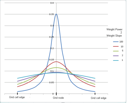
Normalized weight curves W = 1/(D p+S -1)
Controlling Grid Accuracy
The gridding algorithm combines the observed data points within each grid bin to produce a single initial value for each grid node. A system of differential equations that defines a minimum curvature surface is then numerically solved so that at best it crosses the initial grid node values and at worst comes within the specified tolerance of the grid nodes.
The accuracy of the resulting grid is defined by how closely the solution surface matches the initial values and is controlled by the two parameters: Tolerance and % Pass tolerance.
The tolerance is actually the minimum value of the largest change in the grid from one iteration to the next. When the change is below the minimum value, the iteration process stops. Therefore, it is not a direct measure of the accuracy of the fit to the data. It is usually best to make it very small so that the iteration process is controlled by the maximum number of iterations.
The advantage of tightening the tolerance is to generate a grid that follows the observed data more accurately. However, this sometimes can produce a grid with higher frequency features. A few factors have to be considered when choosing the tolerance parameters, including the type of data, the data coverage, and the scale at which the interpretation is performed.
Adjusting Gridding Algorithm Settings
Maximum Iterations (RANGRID.ITRMAX)
The purpose of this setting is to reduce the processing time; however, it is recommended to increase the value so that the tolerance criteria are met first. By default, this parameter is set to 100; you can easily increase it to as much as 500 without noticing much process time degradation. Higher values of this setting tend to produce more accurate grids. At each greater coarseness level, the value of the maximum iterations setting is reduced by a factor of 2. As it is doubled each time the cell size is halved in the RANGRID process, its default value for an initial coarsest grid (ICGR = 8) is 12. If ICGR = 16, ITRMAX will be only 6, which is too small and ITRMAX should be increased to at least 200 in that case.
Starting Coarse Grid (RANGRID.ICGR)
The starting coarse grid setting defines the desired coarseness of the starting fitting level. Since at each level the grid cell size is halved, this setting is defined as a 2n multiple of the final grid cell size. By starting with a coarser grid, the algorithm can produce a reasonable result in under-sampled areas. As the coarseness decreases, the algorithm becomes more sensitive to high-frequency features in the data.
The initial coarse grid ratio should give an initial grid size that is not less than about 1/4 of the maximum data spacing or gap. For gridding a 200m spaced gravity survey with 10 km spaced regional data, ICGR should be set to 16. For typical aeromagnetic data, a value of 1 would be adequate. However, this might well be much slower than using the default value since every grid point would need to be assigned an initial value by the weighted means method, which is very slow for a large number of data points, instead of one in 64.
This parameter is used while processing the initial coarse grid. Initial values are assigned to the coarse grid based on the weighted mean of data within the search radius of each grid point. If the search radius is too small, the starting grid can be a poor approximation of the desired grid resulting in excessive processing time. If the search radius is too large, too much time might be consumed establishing the original coarse grid.
When gridding densely sampled data, you may want to decrease the value to save processing time When gridding spare datasets, you may want to increase the value to avoid situations where no data points are found within the defined radius from a grid node.
It is critical that you choose the search radius large enough to give at least one data point within the search radius of every one of the coarse grid nodes. Otherwise, the initial value assigned to it (global average) may be too far from the solution for it to iterate to its correct value. The default is usually large enough – except when there are very large gaps in the data relative to the cell size. This exception can occur when the gridding detailed surveys together with regional data.
Overcoming Poorly Sampled Data
Although a minimum curvature surface may be mathematically ideal, it is not well suited to under-sampled data. Data is said to be under-sampled when the sample density is not sufficient to define all details of the feature(s) being sampled. In theory, sampling should be at half the size of the smallest feature present. Note that this is half the smallest feature present in the data, not half the smallest features of interest. This is an important distinction because many types of data often contain noise, that is much smaller spatially than the features of interest. This noise can be comparable or larger in amplitude than those features of interest. If this noise is under-sampled, error (known as aliasing) can be introduced into the data. The higher the amplitude of the noise, the more significant the error.
In practice, the cost of data is roughly proportional to the number of samples. Because of this, many data sets, if not most data sets, are undersampled in order to reduce cost. These data still contain useful information, but must be handled by the gridding process in such a way that aliased noise is minimized. Minimum curvature gridding (RANGRID) has two features, which the user can control to minimize this type of error: the low-pass de-aliasing filter and the internal tension.
A dealiasing filter is a low-pass (smoothing) filter designed to remove high frequency noise in the data before gridding. In minimum curvature gridding, this is controlled by averaging data to a single point within the vicinity of a multiple of the grid cell size (determined by the de-sampling factor), which effectively produces a boxcar low-pass filter. By default, this multiple is 1 and any sampling finer than one grid cell in dimension is averaged. This multiple can be increased to produce more smoothing as desired.
Dealiasing filters are particularly useful when sampling is uneven. In such surveys the widest distance between adjacent sample points defines the sampling limit. A suitable low-pass filter should be set to at least the wavelength defined by this distance.
For example, a data set may be well sampled at a nominal 500-meter sample interval and include some lines sampled at 10 metres or locally dense sampling at 50 metres. In this situation, the limiting sampled distance is 500 metres. If a 100-meter grid is to be produced, the desampling factor in the minimum curvature gridding should be set to 5.
However, there are weaknesses to this method. If a noise spike happened to be located at one of the more coarse 500-meter observation points, the minimum curvature gridding will produce an erroneous feature at that location because that noise is not sufficiently sampled. This is unavoidable aliasing noise for which the only solution is increased sample density. When reviewing gridding results critically, be suspicious of features defined by only one observation point unless you are confident that local noise does not exist.
Another weakness becomes apparent when you are interested in spatially smaller features that are locally well sampled within a more coarsely sampled background. Applying a dealiasing filter based to the coarse samples causes too much smoothing in the detailed areas, whereas applying too little filtering can produce severe overshooting beyond the detailed data. Increasing tension as described in the next section can overcome some of the overshooting, but this also tends to increase bulls-eye effects around the coarser data points.
Apply Internal Tension
Minimum-curvature surfaces can be viewed as elastic plate flexures; they approximate the shape adopted by a thin plate flexed to pass through the data points. Minimum-curvature surfaces may have large oscillations and extraneous inflection points in sparsely sampled regions. These extraneous inflection points can be eliminated by adding tension to the elastic-plate flexure equation; thus improving the convergence of the iterative method of solution for the gridding equations. If you notice localized highs and lows in areas of sparse coverage, you would have to increase the tension to eliminate this artefact of gridding.
Overshoot in unconstrained areas
In general, overshooting in unconstrained areas may be a result of one of:
1. A poor minimum curvature solution
The minimum curvature solution may be far from an ideal fit if the starting or coarse grid was not a good approximation of the final grid, or the XYZ data set contained too few points to rapidly pull in the grid during the iteration process. To compensate for this, reduce the tolerance (tol) and, if necessary, increase the number of iterations (itrmax).
2. A good minimum curvature solution
In situations of uneven spacing or insufficient sampling of features, minimum curvature gridding tends to overshoot the observed data points and produce anomalous highs or lows between observation locations. Although this is mathematically ideal and, in some cases, more desirable, it is often the result of poor sampling. The minimum curvature gridding includes the ability to reduce overshoots by the application of internal tension as described by Smith and Wessel (1990). Tension can be thought of as adding springs to the edges of a flat sheet that is forced to go through each data point. If the springs have no tension, a minimum curvature surface results. Increasing tension on the springs begins to flatten the surface such that each data point becomes to a 'tent pole' over which the surface is stretched. Infinite tension produces a straight line in the surface between data points.
The effect of tension on some simple random data is shown in the following figure:
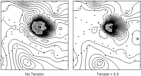
Although the application of internal tension can reduce or eliminate overshoot, it does cause the curvature of the surface to increase in the vicinity of the data points. If the gridded data is to be used in subsequent high frequency processing, such as the calculation of residuals or vertical derivatives, bullseyes around data points become pronounced. Again, the only effective solution to this type of problem is sufficient sampling to allow gridding without tension.
Random Gridding Line Data
Although the minimum curvature gridding (RANGRID) is designed for randomly located data, it may also be used to grid line based data. This is sometimes desirable in situations where line data does not possess a predominant geological trend or where the data from tie lines and baselines is to be included in the gridding.
If line data is to be gridded using RANGRID, the blanking distance should be set to just greater than the maximum line separation. The resulting grid will extend beyond the edges of the data by this distance.
If this is undesirable, you can grid the same data by using bi-directional gridding (BIGRID) to create a mask grid that stops at the edges of the data. The GRIDBOOL GX can then be used to mask off the dummy areas defined by the BIGRID grid. For more information on bi-directional gridding and grid masking refer to the Bi-directional Gridding and GRIDBOOL GX documentation.
For further information on working with the minimum curvature gridding parameters, check the Oasis montaj Fundamentals course at
Got a question? Visit the Seequent forums or Seequent support
© 2023 Seequent, The Bentley Subsurface Company
Privacy | Terms of Use