
Grid Data - Inverse Distance Weighted
Gridding refers to the process of interpolating data onto an equally spaced “grid” of cells in a specified coordinate system. For an introduction to gridding and a summary of the different gridding methods click here.
Inverse Distance Weighted Gridding
Use the Grid Data option from the Grid and Image > Gridding menu to grid data using the Inverse Distance Weighted (IDW) algorithm.
The IDW algorithm calculates a value for each grid node by examining surrounding data points that lie within a user-defined search radius. The node value is calculated by averaging the weighted sum of all the points, where the weighting inversely corresponds to distance from the grid node. It is usually applied to highly variable data (e.g. geochemistry data).
The IDW gridding method is suitable for randomly oriented data with a relatively large number of samples or data collected along specific directions, such as borehole data. It is primarily used to interpolate data where nearby data points are expected to influence one another and it works well with geochemical data.
Inverse Distance Weighted – Gridding Options
|
Data to grid |
Select the database channel to grid. To specify an array element, append to the channel array name the element index in square brackets. For example, Chan[1] would indicate the second element of the array channel "Chan". Script Parameter: IDW_GRIDDING.CHANNEL |
|
Output grid |
Provide the name of the output grid file. This field is auto populated based on the active database and the selected channel to grid; however, you can override the default. The default output grid format is selected automatically as the output file type. The type can be controlled using the browse dialog, which is accessible from the [...] button. Script Parameter: IDW_GRIDDING.GRID |
|
Gridding method |
The current gridding method is displayed. Script Parameter: GRIDDING_TOOL.METHOD [IDW = "3"] |
|
Cell size |
Specify a cell size for the output grid. This field is auto-populated with the calculated default grid cell size and rounded to the nearest ten or hundred: The grid cell size (the distance between grid points in the X and Y directions) should normally be ¼ to ½ of the line separation or the nominal data sample interval. If not specified, the data points are assumed to be evenly distributed, and the area rectangular. The default cell size is then defined by the following formula:
Where:
Script Parameter: IDW_GRIDDING.CELL_SIZE |
Extents and Data |
|
Spatial Extents |
|
|
Grid extents |
Define the spatial limits of the area to be gridded. By default, these fields are set to the full extents of the current X & Y channels of the active database in order to include all the data in the database:
To grid a subset of the data, enter the limits of the bounding rectangle, or press the Draw Extents button to interactively define the boundary extents – the output grid coverage will extend to these limits. Script Parameter: IDW_GRIDDING.XY |
|
[Draw Extents] |
Press this button to interactively define the grid boundary extents: in the Grid Preview pane, use the mouse to click & drag to draw a box, then release the mouse cursor to accept the final size of the box. The X & Y values will be updated in the Grid extents fields, and the preview window will be refreshed to show the newly defined extents. |
|
[Reset Extents] |
Press this button to reset the grid extents to the initial state of defaults for the active database. The Grid Preview pane (when Auto-refresh is enabled) will be updated to reflect the change; however, the zoomed state (in/out) of the grid preview will not be affected.
|
|
Blanking distance |
Specify a blanking distance or leave the auto-populated value, which is calculated as four times the default cell size value (4*Cell size). The blanking distance controls how far the grid is extrapolated away from the nearest data point. All values at distances greater than the blanking distance are set to dummy. Script Parameter: IDW_GRIDDING.BLANKING_DISTANCE |
|
Cells to extend beyond data |
This is the number of grid cells to extend beyond the outside limits of the data. If the default is preserved (set to zero), the grid extents are limited to just overlapping the most extreme data value locations in X and Y. Set this to a number greater than zero to allow the grid to be extrapolated beyond the data edges. The actual extrapolation distance is determined by the Search radius value and limited by the Blanking distance value, and cells extended beyond this distance will remain dummies in the output grid. Script Parameter: IDW_GRIDDING.CELLS_TO_EXTEND (Default: 0) |
Data Filtering |
|
|
Mask channel |
Select a channel from the drop-down list to act as a mask. Only database channels that have the class property set as "MASK" are listed. Additionally, string channels and channels with array size greater than 1 are omitted from the list. The data values in the selected Data to grid channel with corresponding dummy (*) values in the Mask channel will not be used in the gridding process. The X & Y values will be updated in the Grid extents fields to reflect the masked data, and the generated masked grid (with the correct extents) will be automatically rendered in the Grid Preview window (the Auto-refresh option must be selected). Script Parameter: IDW_GRIDDING.MASK_CHANNEL |
|
Log option |
You can either grid the original data or its logarithmic (base 10) representation. Gridding the log of the data can be a very effective way to reduce distortion due to highly skewed data such as geochemical data. The options are:
See the Application Notes below for more details. Script Parameter: IDW_GRIDDING.LOG_OPTION |
|
Log minimum value |
If gridding in log space (see the Log options above), this parameter specifies the minimum value. The default is 1. See the Application Notes below for more details. Script Parameter: IDW_GRIDDING.LOG_MINIMUM (Default: 1) |
Interpolation |
|
Inverse Distance Weighted |
|
|
Search radius |
Enter a value for the search radius or leave the calculated default, which is determined based on the number of cells in X and Y as at least four times the Cell size value. For each grid centre point, all values within the search radius are included in the weighted average yielding the value at that points. If no value is entered, the calculated default is used. Script Parameter: IDW_GRIDDING.SEARCH_RADIUS |
|
Weighting power |
Specify a value greater than or equal to zero. The default value is 2. This parameter modifies the shape of the inverse distance-weighting function. See the definition of the Weighting Slope and Power in the Application Notes below. Script Parameter: IDW_GRIDDING.WEIGHT_POWER (Default: 2) |
|
Weighting slope |
Specify a value greater than or equal to zero. The default value is 1. This parameter modifies the steepness of the inverse distance-weighting function. See the definition of the Weighting Slope and Power in the Application Notes below. Script Parameter: IDW_GRIDDING.WEIGHT_SLOPE (Default: 1) |
|
|
|
|
[Restore Defaults] |
This button remains disabled until any of the fields default values are changed. Press the button to reset the gridding parameters to the initial state of defaults for the active database. When Restore Defaults is clicked: The following parameters are reset to their default values:
The following parameters are not reset:
The Grid Preview (with Auto-refresh enabled) and Variogram panes will be updated to reflect any parameters changes; however, the zoomed state (in/out) of the grid preview will not be affected. |


Application Notes
It is recommended that your first attempt at gridding should use the intelligent defaults. After inspecting the outcome, however, you may decide to modify defaults such as the weighting power and weighting slope, to alter the degree of influence of contributing data points relative to their distance or the blanking distance to fill in the gaps, or to generate the output on logarithmic scale.
Once a gridding task is executed, the gridding options are retained when switching between different databases. The Grid Data tool will recall the previous gridding parameters associated with the current database, regardless of whether gridding tasks have been performed on different databases since.
Log Options
If the data range is very wide and spans over several orders of magnitude, gridding in normal space may not honour the data distribution of interest, and the real patterns present in the data may get obscured in the process of gridding. If, however, the data is gridded in logarithmic space these very patterns will be revealed. Often it is more appropriate to grid geochemical data in logarithmic scale, as the element distribution changes in concentration by orders of magnitude over a short distance. Furthermore, depending on the data concentration and scatter, in order to maintain a consistent texture, it may be more appropriate to display the extremes of the data distribution in logarithmic space while the median range remains in linear space. This would be an appropriate approach with bimodal data.
Highly skewed data, such as geochemical data, can present a problem due to the disproportionate effect that high data values have on the surrounding region. For example, in a geochemical survey where the majority of chemical concentrations are in the range of not detectable to 100 ppm, the odd reading of many thousand ppm becomes weighted too strongly.
To overcome this effect, you can use the logopt parameter to take the log of the data before gridding. Once the data is gridded, you have the option of either restoring the original linear data scaling, or storing the logarithmic data in the output grid.
Logarithmic grids can be contoured by CONTOUR by selecting the logopt parameter in the CONTOUR control file. This option causes CONTOUR to expand any label numbers back to a linear scale before plotting the label. Note that the contour intervals must be selected logarithmically. The most typical logarithmic plot would use two contour levels, 0.25 and 1. Only the 0,1,2,3... levels would be labelled, and CONTOUR would label them 1,10,100,1000...
The log-linear options are not appropriate for geochemical data; they are intended for levelled geophysical data (e.g., sometimes the span of magnetic data is quite broad and in order to be able to observe the definition around the mean of the data distribution as well as at the extremes, this option is used). Prior to gridding the data for the two log-linear options, the data is altered as follows:
if ( Z > Log_minimum)) Z = (log10( Z / Log_minimum) + 1.0) * Log_minimum); if ( 0 < Z ≤ Log_minimum)) Z is untouched if ( -Log_minimum ≤ Z ≤ 0)) Z = -Z if ( Z < -Log_minimum)) Z = -(log10( -Z / Log_minimum) + 1.0) * Log_minimum); |
This has the effect of treating large positive or negative values like logarithms, but gives a linear transform for values around zero.
Log minimum value: when gridding in log space, this setting specifies the minimum cut-off in linear space. If one of the log, save as options has been selected, all values below this cut-off are replaced by Log_minimum. If one of the log-linear,save as options has been selected, this entry represents the two boundaries where the switch between linear and logarithmic gridding occurs.
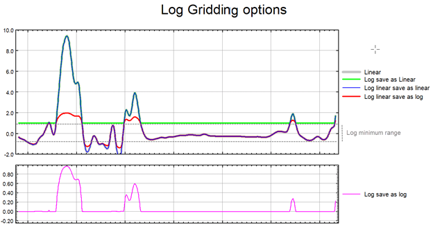
The illustration above intends to convey the variation between the various log options.
Anti-aliasing
Prior to gridding (and after any log or log-linear transformation), data is pre-processed using an anti-aliasing technique. All values falling inside any single grid cell are averaged, and the data is then represented by the single averaged value at the grid cell centre. Any error in the spatial representation of features introduced by this step will never exceed one-quarter of the Nyquist wavelength, which is equal to two cell sizes.
Weighting Slope and Power
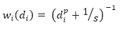
The inverse distance weighting is a deterministic method for multivariate interpolation using a known set of data values at known locations. The grid values at each x,y point are calculated using a weighted average of the known data values within the defined search radius. The weight attributed to each known data value is inversely proportional to its distance from the grid x,y point. Applying a power to the weights will modulate the influence of each known data value as a function of distance. Furthermore, adding a slope factor moderates the sharpness of the weights and prevents them from reaching a large dynamic range in close proximity to the x,y point. The weight of each of the n points within the search radius centered on a point x,y, is defined by the equation:
These weights must be normalized. The normalized weight equation becomes:
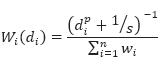
Where:
di is the distance of each of the n known data values gi within the search radius from the grid point x,y
n is the total number of gi values within the search radius
p is a constant power
s is a constant slope
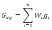
At each grid cell x,y, the value will be calculated as:
Where:
Gxy is the output grid value at location x,y
gi is the input data values within the search radius

The normalized weights (legend) of all gi data points (indicated within the search radius) are calculated. Points outside the search radius are ignored. Then, equation Gxy=∑ni=1Wi gi is applied.
Using a default power of 2 and a slope of 1, produces a standard Gaussian bell-shaped weighting function. A slope > 0 ensures that the weight remains finite at zero distance. Decreasing the slope tends to flatten the bell, resulting in greater weighting of points away from the grid cell, and hence greater smoothing.
A power < 2, or a slope <1, may result in over-smoothing the data.
The following table shows the effect of various slopes on the weighting given at various distances away from the centre cell. The weights have been normalized so the weight at the cell centre is equal to 1
|
|
weighting of centre cell |
weighting 1 cell away |
weighting 2 cells away |
weighting 3 cells away |
weighting 4 cells away |
|---|---|---|---|---|---|
|
P = 2, S = 0.2 |
1 |
0.83 |
0.55 |
0.36 |
0.24 |
|
P = 2, S = 0.5 |
1 |
0.67 |
0.33 |
0.18 |
0.11 |
|
P = 2, S = 1 |
1 |
0.5 |
0.2 |
0.1 |
0.056 |
|
P = 2, S = 2 |
1 |
0.33 |
0.11 |
0.053 |
0.03 |
Clearly, as the slope increases, the weighting is more tightly concentrated about the centre cell. The search radius should also be chosen based on the fall-off of the weighting function. Increasing the search radius beyond where the weighting function is significant, will have little effect on the results, and may result in large increases in processing time, since the processing time varies in proportion to the cube of the search radius. (Remember that the search radius is specified in ground units, not as a multiple of cell sizes).
Got a question? Visit the Seequent forums or Seequent support
© 2023 Seequent, The Bentley Subsurface Company
Privacy | Terms of Use