Display Radial Spectrum

Use the 2D Filtering > Display Radial Spectrum option (FFT2SMAP GX) to create a spectrum profile map from the *.SPC file generated by MAGMAP.

Display Radial Spectrum dialog options

Input spectrum file

Specify the name of the input spectrum file. Script Parameter: FFT2SMAP.SPEC

Application Notes

Mathematically, the Fourier transform of a space domain function f(x,y) is defined as:

The reciprocal relation is:

Where μ and ν are wavenumbers in the x and y directions, respectively, measured in radians per metre if x and y are in given metres. These are related to spatial frequencies ƒ_x and ƒ_y, in cycles per metre.

A grid (in the space domain) is transformed to and from the wavenumber domain using Fast Fourier Transform (FFT). The equivalent data set in the wavenumber domain is commonly called “Transform”. A Transform of a grid is composed of wavenumbers, which have units of cycles/metre, and have a real and imaginary component. Just as a grid samples a space domain function at even distance increments, the Transform samples the Fourier domain function at even increments of 1/(grid size) (cycles/metre) between 0 and the Nyquist wavenumber (1/[2*cell size]).

A given potential field function in the space domain has a single and unique wavenumber domain function, and vice versa. The addition of two functions (anomalies) in the space domain is equivalent to the addition of their Transforms.

The energy spectrum is a 2D function of the energy relative to wavenumber and direction. The radially averaged energy spectrum is a function of wavenumber alone, and is calculated by averaging the energy for all directions for the same wavenumber.

The Fourier transform of the potential field produced by a prismatic body has a broad spectrum whose peak location is a function of the depth to the prism’s top and bottom surfaces, and whose magnitude is determined by the prism’s density or magnetization. The peak wavenumber (ω’) can be determined by the following expression:

Where:

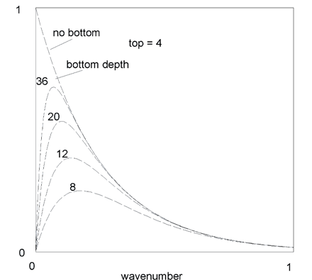
The spectrum of a bottomless prism peaks at the zero wavenumber according to the following expression (Bhattacharya, 1966):

Where h is the depth to the top of the prism.

The spectrum for a prism with top and bottom surfaces is:

Where h_t and h_b are the depths to the top and bottom surfaces, respectively. As the prism bottom is brought up, the peak moves to higher wavenumbers as illustrated in the following figure:

Considering the spectrum of a fixed-size prism, as the prism depth is increased, the peak of the spectrum is shifted to lower wavenumbers (the anomaly becomes broader), and the magnitude of the spectrum is reduced.

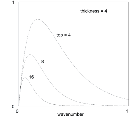
An important fact to note in the above figure is that the spectrum of a deep prism does not exceed the magnitude of the same prism at a lesser depth at any wavenumber – only the peak is shifted to lower wavenumbers. Because of this, there is no way to separate the effect of deep sources from shallow sources of the same type using wavenumber filters. This is only possible if the deep sources are of stronger magnitude, or if the shallow sources have a lesser depth extent.

When considering a grid that is large enough to include many sources, the logarithmic spectrum of this data can be interpreted to determine the statistical depth to the tops of the sources using the following relationship:

The depth of an ensemble of sources is easily determined by measuring the slope of the energy (power) spectrum and dividing it by 4π. A typical energy spectrum for magnetic data may exhibit three parts – a deep source component, a shallow source component, and a noise component.

The following figure illustrates the division of an energy spectrum into these three components:

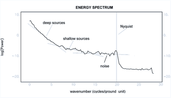
Matched Filtering helps determine the slope of these 3 regions and produces the equivalent depth slices.

MAGMAP is commonly used to enhance information of interest in a given 2D data set, either by removing features considered as “noise”, or by enhancing the features of interest. For example, if you are interested in shallow features in a magnetic map, you might apply a first or second vertical derivative filter to the data in order to enhance shallow features at the expense of anomalies caused by deeper sources.