Free Air and Bouguer Anomaly

Use the Gravity > Free Air, Bouguer Anomaly menu option (geogxnet.dll(Geosoft.GX.Gravity.FreeAirAndBouguerAnomaly;Run)*) to carry out the following components of a gravity reduction:

(i) Free Air anomaly calculation

(ii) Bouguer anomaly calculation

(iii) Complete Bouguer anomaly (Bouguer anomaly + terrain correction)

Free Air and Bouguer Anomaly dialog options

Database	The name of the current database (displayed for information only).
Corrected gravity channel	Select the gravity corrected channel (in milligals). Script Parameter: GRAVRED.GRAVITY
Terrain correction channel	Select the terrain correction channel. By default, if there is a channel named "Terrain" in the database, it will be selected. Script Parameter: GRAVRED.TCORCH
Terrain correction density	The default terrain density (in g/cm³) is set to the last terrain density used to calculate the terrain effect. You can, however, override this density if necessary. Should you opt to calculate multiple Complete Bouguer anomalies in a single run, for each density, the terrain effect channel data is rescaled using the provided correction density prior to be added to the output gravity channel. It is important to note that if the terrain effect is calculated near bodies of water, the density variability is not taken into account. In such instances, for each density, the terrain correction must be calculated separately. See the Complete Bouguer Anomaly section in the Application Notes below. Script Parameter: GRAVRED.TDENST
Elevation channel	Select the elevation channel. By default, if there is a channel named "Elevation" in the database, it will be selected. Script Parameter: GRAVRED.ELEVATION
Output free air anomaly channel	Specify the name of the output free air anomaly channel. Normally, this should be placed in channel "FreeAir"; however, you have the option of changing the name. Script Parameter: GRAVRED.FREEAIR
Free air correction method	Select an elevation correction formula from the list: 0.308596 mGal/m 0.3086 mGal/m (Sheriff) Ellipsoid (Heiskanen & Moritz) - the full ellipsoid expression as a function of height and latitude from Heiskanen and Moritz [1]. Additional elevation correction formulas can be defined and stored in the file named "Gravity_Free_Air.lst" located in the %USERPROFILE%\Documents\Geosoft\Desktop Applications \etc directory. Script Parameter: GRAVRED.FREE_AIR
Apply Bullard (Bullard B) correction	Check this option to apply the curvature correction to the Bouguer anomaly. Script Parameter: GRAVRED.CURVATURE [1 – Yes (default) | 0 – No]
Latitude channel	This is a contextual parameter. If the Free air correction method selected is "Ellipsoid (Heiskanen & Moritz)", or the option Apply Bullard (Bullard B) correction is checked, you will be prompted to provide the latitude channel required for the free air correction. By default, if there is a channel named "Latitude" in the database, it will be selected. Script Parameter: GRAVRED.LATITUDE
Output Bouguer anomaly channel	Specify the name of the output Bouguer anomaly channel. Normally, this should be placed in channel "Bouguer". You have the option of changing the name in case you wish to create a number of Bouguer anomaly channels with different earth densities. Script Parameter: GRAVRED.BOUGUER
Number of Bouguer corrections	Specify the number of Bouguer corrections. The default is 1. If a number > 1 is entered, you will be prompted to enter a Minimum earth density and a Maximum earth density. Incremental densities will then be calculated, and for each density, a Bouguer correction and Bouguer anomaly will be calculated. The density used for the calculation will be appended to the name of the output channels. Display the Bouguer profiles for these channels, in the database profile window, to decide on the Bouguer correction to use and the optimal density that can best remove the terrain effect. See the Application Notes below for more details on Bouguer anomaly calculation and Nettleton’s method[7]. Script Parameter: GRAVRED.CORRECTION_NUMBER
Earth density (g/cc)	Specify the density of the earth (in g/cm³) for calculating the Bouguer correction. Script Parameter: GRAVRED.DENSITY_EARTH
Minimum earth density (g/cc)	Specify the minimum density of the earth (in g/cm³) for calculating the Bouguer correction. Available when the Number of Bouguer corrections is > 1. Script Parameter: GRAVRED.DENSITY_EARTH_MIN
Maximum earth density (g/cc)	Specify the maximum density of the earth (in g/cm³) for calculating the Bouguer correction. Available when the Number of Bouguer corrections is > 1. Script Parameter: GRAVRED.DENSITY_EARTH_MAX
Other layer	Check this box if you wish to supply water/ice or overburden thickness and densities. Script Parameter: GRAVRED.OTHER_LAYER [1 – Yes (default) | 0 – No] Layer This is a contextual entry. If “Other layer” is checked, you are prompted to define if you are providing an Overburden or a Water layer. By default, the water layer is checked. Water density (g/cc) Specify the density of water to be used for the Bouguer correction for gravity readings over water (on ice or marine surveys). This is a required field if the Water layer option is selected above. The density of fresh water is 1.0 g/cm³; salt water ranges from 1.02 to 1.07 g/cm³. Script Parameter: GRAVRED.DENSITY_WATER Water depth channel The water depth is positive below the gravity station. If the gravity station is on land, the channel depth value would be zero. Script Parameter: GRAVRED.WATER_CHANNEL Ice density (g/cc) This is an optional entry. Specify the density of ice to be used for the Bouguer correction for gravity readings on ice. The density of freshwater ice is 0.97 g/cm³ and varies for sea water. Script Parameter: GRAVRED.DENSITY_ICE Ice thickness channel This is an optional entry. It contains the thickness of ice below the gravity station for calculating the ice correction. The depth of "Water" must include the "Ice" thickness. If provided, the ice density becomes mandatory. Script Parameter: GRAVRED.ICE_CHANNEL Overburden density (g/cc) Specify the density of the overburden to be used for the Bouguer correction for gravity readings over water (on ice or marine surveys). This is a required field if the Overburden layer option is selected. Select this option if the density of the overburden is distinctively different from the surrounding rock and there is a thick overburden layer. Script Parameter: GRAVRED.DENSITY_OVERBURDEN Overburden thickness channel The overburden thickness is positive below the gravity station. Where there is no overburden, set the thickness to zero. Script Parameter: GRAVRED.OVERBURDEN_CHANNEL
[More] Click to view and modify the gravitational constant.
Gravitational constant	Over time, the gravitational constant changes ever so slightly. The default is set to the 2010 Gravitational constant in units of 10−11⋅m3⋅kg−1⋅s−2. See the Gravitational Constant section under Application Notes for further details. Script Parameter: GRAVRED.GRAVITATIONAL_CONSTANT

Application Notes

This GX assumes that:

• a gravity database is currently loaded (see Import Gravity Survey).

• the tide and drift corrections have been applied to produce absolute gravity (see Gravity Corrections).

• the latitude, longitude ground locations are defined.

• the latitude correction (the theoretical gravity at the station location) has been applied (see Latitude Correction).

• the free air anomaly results will be stored in the "FreeAir" channel in the database.

• the survey elevation data should be contained in an "Elevation" channel in the database.

For an Airborne survey, the flight elevation should be provided. For a Shipborne survey, the water depth should be provided.

1. Free Air Anomaly

The free air correction is calculated and added to the latitude corrected gravity. The expressions for the supported corrections are:

Where:

Hs	Station elevation in metres (relative to the datum, positive up)
L	Latitude of the station

The last formula accounts for the non-linearity of the free air anomaly as a function of both latitude and height above the geoid.

Each expression should be defined on one line, and it should consist of a unique name followed by the complete expression using the following syntax:

Where:

Input_Gravity

Variable containing the input gravity channel; designated by the variable $sGravity

In the expression, you can also use the variables:

	Conversion factor used to convert the units of elevation to metres
	Elevation channel
	Latitude channel

For example, the syntax of the standard free air correction equation can be written as:

2. Bouguer Anomaly

Bouguer anomaly corrects the free air anomaly for the mass of rock that exists between the station elevation and the spheroid. It includes a correction for water depth and ice thickness if the "Water" and "Ice" channels are non-zero:

Bouguer Anomaly Correction Formula

For ground survey (including on lake surface) or shipborne (marine) survey:

For airborne survey:

Where:

Gb	Bouguer anomaly in milligals
Gf	Free air anomaly
D	Bouguer density of the earth in g/cm³
Dw	Bouguer density of water g/cm³
Di	Bouguer density of ice in g/cm³
Hs	Station elevation in metres
Hw	Water depth in metres (including ice)
Hi	Ice thickness in metres
Gc	Curvature (Bullard B) correction
Hg	Ground (DEM) elevation at survey station location in metres

Water Channel

The "Water" channel contains the water depth at the gravity survey station location. These depths should be positive or zero.

Curvature (Bullard B) Correction Gc

The purpose of the curvature correction as a step in producing the Bouguer anomaly is to convert the geometry for the Bouguer correction from an infinite slab to a spherical cap whose thickness is the elevation of the station and whose radius (arc length) from the station is 166.735 km. Curvature correction depends on the station elevation (e.g.,1.1 mGal at 1000 m, 1.5 mGal at 2000 m, 1.2 mGal at 3000 m, 0.2 mGal at 4000 m, -1.5 mGal at 5000 m and –3.9 mGal at 6000 m), and latitude (ranging in dozens µGal). LaFehr’s formula [6], is used here for the curvature correction.

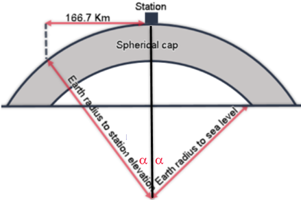
Figure 1: Schematic illustration (not to scale) of the spherical cap in Bullard B correction. The spherical cap surface radius of 166.7 Km, which is the outer radius or the Hayford-Boweie Zone O, is based on minimizing the difference between the effect of the cap and that of an infinite horizontal slab [LaFehr, 1991].

LaFehr expands the Bullard B correction calculation as per below:

Where:

BB: Bullard B correction γ:  Gravitational constant ρ:  Density h:  Elevation (from sea level) R:  Earth radius to the station:          Where:     Ro: Earth’s sea level radius at the survey location μ:  Dimensionless coefficient:     λ: Dimensionless coefficient:            Where:                                                                α =  The half angle subtended at the earth’s center by the section of the earth’s surface at sea level for which the outer distance from the station is normally taken to be 166.7 km.

For context, below is what each of the Bullard corrections refers to:

• Bullard A: approximates the local topography (or bathymetry) by a slab of infinite lateral extent, constant density, and thickness equal to the elevation of the point with respect to the mean sea level.
• Bullard B: curvature correction, which replaces the Bouguer slab by a spherical cap of the same thickness to a distance of 166.735 km.
• Bullard C: terrain correction, which consists of the effect of the surrounding topography above and below the elevation of the calculation point [Nowell, 1999].

3. Complete Bouguer Anomaly

The Complete Bouguer anomaly corrects the Bouguer anomaly for irregularities of the earth due to terrain in the vicinity of the observation point. The terrain correction GXs can be used to calculate the terrain correction.

The complete Bouguer anomaly equation is:

Where:

	The term is calculated in the Gravity Corrections GX
	The term is calculated in the Latitude Correction GX
	The terrain effect at density ρo
	The term is calculated by this GX for all incremental ρo values

Linear Correlation Coefficient

If more than one Bouguer anomaly channel is requested, a Linear Correlation Coefficient is calculated for each density and reported in a popup window. Normally, to select the density that yields the least correlation between the shape of the topography and the calculated Complete Bouguer anomaly, you would visually focus on sections where the topography channel varies a lot (hills & valleys) then check if the gravity follows a similar trend and disregard the correlation in the remainder of the data. With this in mind, to use the Linear Correlation Coefficient as a decision aid, calculate it for such subsets of data. Select carefully a subset where you know that the topography is evident in the gravity data and apply the Bouguer correction for multiple densities. Once you find the best density (least correlation, coefficient closest to zero) use it to calculate the Bouguer anomaly for the entire dataset.

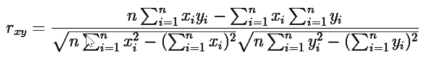
The Linear Correlation Coefficient equation is:

Where:

x	Complete Bouguer anomaly
y	Elevation

The correlation coefficient values reside between -1 and 1. A correlation coefficient closer to 1 indicates a close correlation between the x (Complete Bouguer anomaly) and y (elevation) profiles. A coefficient closer to -1 indicates an inverse correlation. As the coefficient approaches 0, the correlation decreases. The correlation that is the closest to 0 will be indicated with a star symbol (*) – as the least correlated one.

The correlation coefficients for the specified densities are reported at the end of the process. Furthermore, these coefficients are saved in the project working folder under the unique file name: "BouguerNettletonCrossCorrelationCoefficientsyyymmdd.log"

Nettleton’s Method

Nettleton’s method is based on the observation that the use of an appropriate reduction density will remove a correlation of observed gravity with topography. In this method, a gravity profile over a study area, in which there are significant sharp variations in elevation, is reduced by using a range of Bouguer reduction densities. The reduction density with a minimum correlation with elevation would give anomalies most representative of the underlying geologic structure.

The following assumptions must hold for Nettleton's method to apply:

• Nettleton's estimate fails if the topography is dominated by deeper geological structures.
• A relatively homogeneous density distribution in the area of interest.
• Sufficiently large (> 100 m) elevation differences and a uniform distribution of gravity measurements with respect to horizontal positions 'and elevations.
• A sufficient model of the regional field to be separated from the data.

Gravitational Constant

The gravitational constant (G) is a physical constant that is difficult to measure with high accuracy and which has varied broadly over time. G is re-evaluated every four years approximately. The table below lists published figures along with the uncertainty and source.

Published G Values:

Year	G (10−11·m3⋅kg−1⋅s−2)	Standard Uncertainty	Reference
1969	6.6732(31)	460 ppm	Taylor, B. N.; Parker, W. H.; Langenberg, D. N. (1 July 1969). "Determination of e/h, Using Macroscopic Quantum Phase Coherence in Superconductors: Implications for Quantum Electrodynamics and the Fundamental Physical Constants". Reviews of Modern Physics. American Physical Society (APS). 41 (3): 375–496.
1973	6.6720(49)	730 ppm	Cohen, E. Richard; Taylor, B. N. (1973). "The 1973 Least‐Squares Adjustment of the Fundamental Constants". Journal of Physical and Chemical Reference Data. AIP Publishing. 2 (4): 663–734.
1986	6.67449(81)	120 ppm	Cohen, E. Richard; Taylor, Barry N. (1 October 1987). "The 1986 adjustment of the fundamental physical constants". Reviews of Modern Physics. American Physical Society (APS). 59 (4): 1121–1148.
1998	6.673(10)	1500 ppm	Mohr, Peter J.; Taylor, Barry N. (2012). "CODATA recommended values of the fundamental physical constants: 1998". Reviews of Modern Physics. 72 (2): 351–495.
2002	6.6742(10)	150 ppm	Mohr, Peter J.; Taylor, Barry N. (2012). "CODATA recommended values of the fundamental physical constants: 2002". Reviews of Modern Physics. 77 (1): 1–107.
2006	6.67428(67)	100 ppm	Mohr, Peter J.; Taylor, Barry N.; Newell, David B. (2012). "CODATA recommended values of the fundamental physical constants: 2006". Journal of Physical and Chemical Reference Data. 37 (3): 1187–1284.
2010	6.67384(80)	120 ppm	Mohr, Peter J.; Taylor, Barry N.; Newell, David B. (2012). "CODATA Recommended Values of the Fundamental Physical Constants: 2010". Journal of Physical and Chemical Reference Data. 41 (4): 1527–1605.
2014	6.67408(31)	46 ppm	Mohr, Peter J.; Newell, David B.; Taylor, Barry N. (2016). "CODATA Recommended Values of the Fundamental Physical Constants: 2014". Journal of Physical and Chemical Reference Data. 45 (4): 1527–1605.
2018	6.7430(15)	22 ppm	Eite Tiesinga, Peter J. Mohr, David B. Newell, and Barry N. Taylor (2019), "The 2018 CODATA Recommended Values of the Fundamental Physical Constants" (Web Version 8.0). Database developed by J. Baker, M. Douma, and S. Kotochigova. National Institute of Standards and Technology, Gaithersburg, MD 20899.

References

- [1] W. A. Heiskanen and H. Moritz, Physical Geodesy, (San Francisco: W. H. Freeman and Company, 1967).
- [2] R. J. Blakely, Potential Theory in Gravity and Magnetic Applications, (Cambridge: Cambridge University Press, 1995), p. 135.
- [3] R. J. Blakely, Potential Theory in Gravity and Magnetic Applications, (Cambridge: Cambridge University Press, 1995), p. 136.
- [4] R. E. Sheriff, Encyclopedic Dictionary of Exploration Geophysics, 2nd ed., (Society of Exploration Geophysicists, 1984), p. 141.
- [5] R. E. Sheriff, Encyclopedic Dictionary of Applied Geophysics, 4th ed., (Society of Exploration Geophysicists, 1991).
- [6] T. R. LaFehr, "An exact solution for the gravity curvature (Bullard B) correction", Geophysics, vol. 56, no. 8 (1991), pp. 1179-1184. DOI: https://doi.org/10.1190/1.1443138.
- [7] Rémy Villeneuve, "Nettleton's method applied to a field survey", redacted for the course Introduction to Geophysics, (University of Iceland, 2005).
Got a question? Visit the Seequent forums or Seequent support
© 2024 Seequent, The Bentley Subsurface Company
Privacy | Terms of Use