Updates to Previous Versions
- Leapfrog Geothermal 3.6
- Leapfrog Geothermal 3.5
- Leapfrog Geothermal 3.4
- Leapfrog Geothermal 3.3
- Leapfrog Geothermal 3.2
- Leapfrog Geothermal 3.1
- Leapfrog Geothermal 3.0
Leapfrog Geothermal 3.6
- TETRAD Import and Visualisation
- Unstructured TOUGH2 Grids
- Copying TOUGH2 Models
- Static Copies of TOUGH2 Models
- Variable Well Radius Scaling
- Well Trace Object
- acQuire Update
- Mesh Clean Up Improvements
- Reloading Meshes
- Structural Data Analysis
- Graphs and Statistics Refresh
- Cross Section Improvements
- Sub-Blocked Model Export Improvements
- DWG Export
- Hyperlinks in Comments and Notes
- Central Publishing Improvements
- Single Sign-In for My Leapfrog and View
- Inclination for Survey Measurements
- Changes to Flow Modelling Organisation
TETRAD Import and Visualisation
TETRAD flow simulation models can now be imported into and visualised in Leapfrog Geothermal.
See TETRAD Models for more information.
Unstructured TOUGH2 Grids
It is now possible to create a TOUGH2 flow model with an unstructured grid geometry with well locations, faults and other objects as control features. The grid is an unstructured Voronoi grid in x,y and layered in z.
See Unstructured TOUGH2 Models for more information.
Copying TOUGH2 Models
It is now possible to copy a TOUGH2 model in the project tree. Both imported models and those created in Leapfrog Geothermal can be copied.
When an internally created TOUGH2 model with an unstructured grid is copied, the copy is fully dynamic and both the grid geometry and the assignment of rock types to the grid can be modified.
Static Copies of TOUGH2 Models
It is now possible to make a static copy of a TOUGH2 model that has been created in Leapfrog Geothermal. The grid geometry in a static TOUGH2 model cannot be changed. However, if the geological model associated with the TOUGH2 model is modified, the rock type table and the assignment of rock types to the grid blocks will be updated.
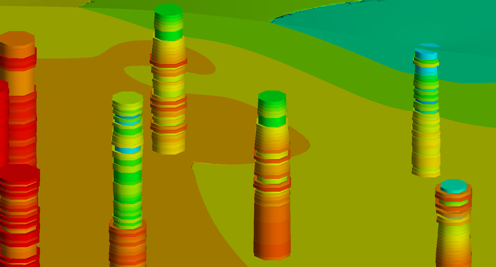
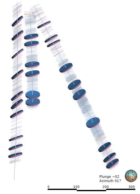
Variable Well Radius Scaling
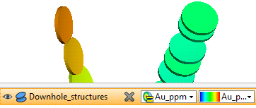
When visualising downhole numerical data you can now scale the width of the well cylinder by another column of data values from your well database.
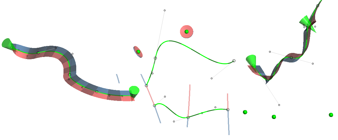
Well Trace Object
There is a new Well traces object in the Wells folder that allows for independent display of well traces in the scene:
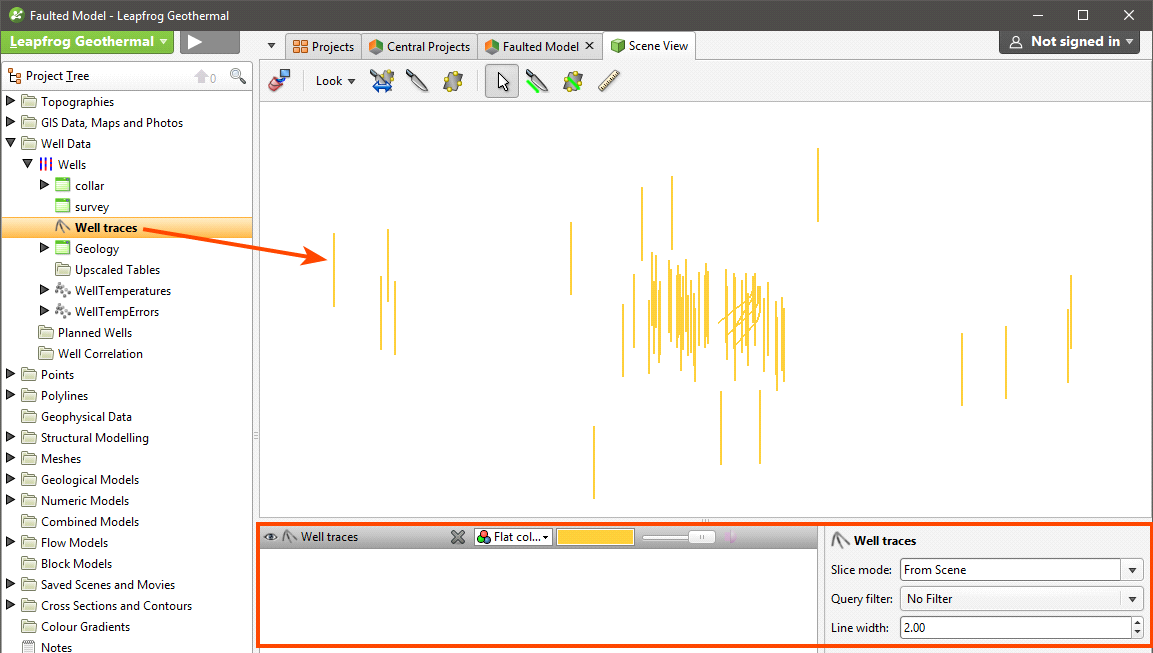
Traces can be displayed using a flat colour that can be changed using the shape list. Trace display properties can be changed in the properties panel.
acQuire Update
The acQuire API has been updated to make loading and refreshing well data easier. This includes the introduction of acQuire’s Smart Refresh. Smart Refresh obtains the latest drilling data from the acQuire database without having to reload the entire contents of the database. This can greatly reduce the amount of data transfer and so speed up data updates. Smart Refresh will only include wells relating to data that has been changed since the database was last updated in Leapfrog Geothermal.
See Connecting to an acQuire Database for more information.
Mesh Clean Up Improvements
Surfaces and imported meshes may have overlapping triangles (known as self-intersections) that prevent the mesh from being usable in further mesh operations. An option has been added to remove self-intersections. See Cleaning Up a Mesh for more information.
Reloading Meshes
Meshes imported into Leapfrog Geothermal and created from extracting mesh parts can now be reloaded. Right-click on the mesh, select Reload Mesh, then navigate to the file that should be used.
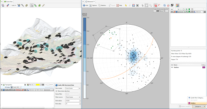
Structural Data Analysis
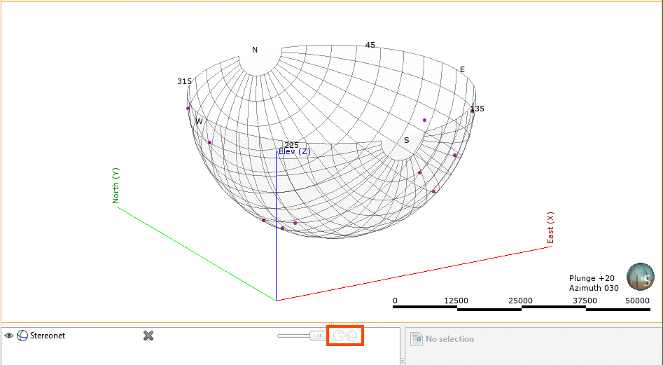
The statistics displayed for stereonets has previously been limited to Fisher statistics, which are calculated for polar data. In addition, it was not possible to view statistics on structural data or lineations in the project tree. Bingham statistics, which are more useful for folded geologies, are now available. The addition of Bingham statistics has resulted in several changes to stereonets. The first is the addition of two new buttons in the stereonet toolbar and the removal of the Statistics button.
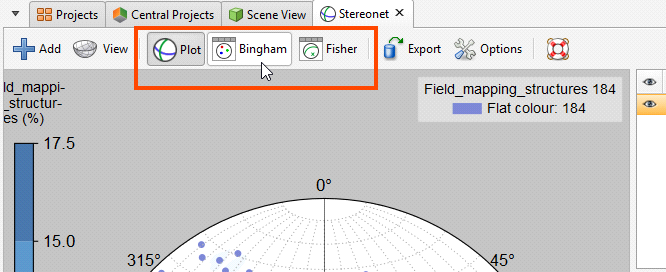
Clicking the Plot, Bingham and Fisher buttons switches between the display of the stereonet and the statistics tables.
You can also view statistics on structural data tables and lineations.
See Stereonets and Viewing Statistics on Structural Data for more information.
Graphs and Statistics Refresh
A Table of Statistics option has been added to Statistics. Together with other improvements, this provides more options and controls when working with statistics and graphs.
- Multiple categories can be populated and grouped
- Statistics columns can be selected
- Both interval length-weighted and un-weighted statistics can be displayed
- Query filters can be applied
- Histograms can be accessed directly from the numeric data column
- Data shown in plots is linked to data in the 3D scene so that you can select in the plot and visualise the selected dataset in the scene, and vice versa
See Statistics for more information.
Cross Section Improvements
A number of improvements have been made to the section editor, including:
Line Evaluations
See Section Layouts for more information.
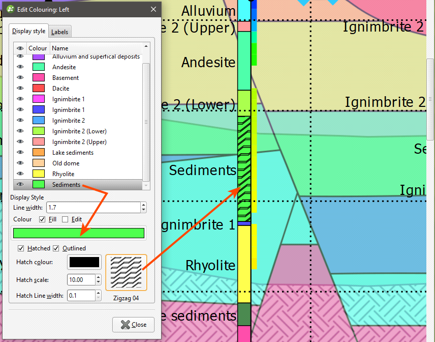
Hatching on Wells
When laying out cross sections it is now possible to display hatching on wells.
See Adding Styling Wells and Planned Wells for more information.
Arrange Labels on Cross Sections
Where multiple wells are evaluated in a confined space, cross section layouts can become hard to read or even overlap. Now it is easy to arrange the collar labels into a custom composition by simply dragging the collar labels to the desired location.
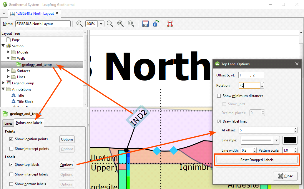
See Adding Styling Wells and Planned Wells for more information.
Sub-Blocked Model Export Improvements
The advanced block model export introduced in Leapfrog Geothermal 3.5 has been added to sub-blocked models exported in Datamine format.
DWG Export
DWG is now available as an export format for:
- Sections
- Serial sections
- Points
- Numeric model values
- Polylines
- Meshes
DWG export uses the same data in the same hierarchical format used for DXF export.
Hyperlinks in Comments and Notes
Comments and notes in Leapfrog Geothermal projects now support hyperlinks. URLs entered in comments and notes will automatically be hyperlinked.
Central Publishing Improvements
It is now possible to publish more types of data to Central, including downhole points, GIS data, images, textures, cross sections and polylines.
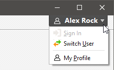
Single Sign-In for My Leapfrog and View
There is a new menu in the upper right-hand corner of the Leapfrog Geothermal window that lets you sign in to My Leapfrog and View:
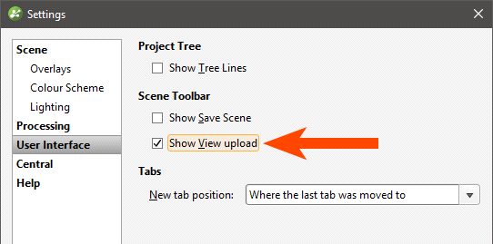
Because how you sign in to View has changed, the settings that were in the View panel of the Settings screen are no longer necessary. There is a new option in the User Interface panel, Show View upload:
Inclination for Survey Measurements
Leapfrog Geothermal now supports inclination values in the survey table when importing well data. It is not possible to import both an inclination column and a dip column, so if a table contains both columns, you will need to choose between the two.
See The Survey Table for more information.
Changes to Flow Modelling Organisation
How flow models appear in the project tree has been reorganised. Options available by right-clicking on the Flow Models folder are now organised by type of model. In addition the term “Structured Model” is now used for MODFLOW.
Leapfrog Geothermal 3.5
- Data Analysis Tools
- Numeric Point Upscaling
- New Faulted Rocktype Evaluation in TOUGH2
- TOUGH2 In-scene Property Display
- Vein Reprocessing Improvements
- Combine Identical Vertices
- Block Model Export Options
- Category Selection on Downhole Points
- Import Meshes From Central
- View Integration with Leapfrog Geothermal
Data Analysis Tools
There are two new data analysis tools in Leapfrog Geothermal, Graphs and Compositing Comparison.
Graphs
The first of the new statistical graph configurations describes and illustrates univariate statistics on numeric columns, including interval length, in one complete window. Several options, including a separate and exportable summary table, manual axis limits and bin width controls, will have a significant impact on the usability of this feature.
A key feature in how the graph interacts with the scene opens a multitude of options, e.g. categorising data in the 3D scene that has been analysed and scrutinised in the graph. A sharp look and feel to the presentation provides a report-ready appearance.
See the Analysing Data topic for more information on the types of graphs available.
Compositing Comparison
Comparing grade distribution or interval length before and after compositing requires a specialized graph to guide important decisions. This new bivariate histogram for composited data, displays raw and composited data on a single graph. A table of summary statistics directly compares populations, providing a full picture of the effect of a particular compositing approach has had on the data distribution.
Numeric Point Upscaling
There is a new tool for well log upscaling available in Leapfrog Geothermal 3.5, the numeric point upscaling tool. This works with downhole points, such as LAS points. See Numeric Point Upscaling.
New Faulted Rocktype Evaluation in TOUGH2
Faults typically have a crush zone that affects the flow properties of the surrounding rock. Modelling fluid flow inside a fault is an important aspect of creating a reservoir model, which is why a new faulted rocktype evaluation has been added to TOUGH2 models. This evaluation is based on the fault system of the geological model associated with the TOUGH2 model. For TOUGH2 models created in Geothermal, the faulted rocktype evaluation is automatically created when the TOUGH2 grid is defined; for imported TOUGH2 grids, the evaluation is created when rocktypes are generated for the grid.
See Evaluating a Faulted Model.
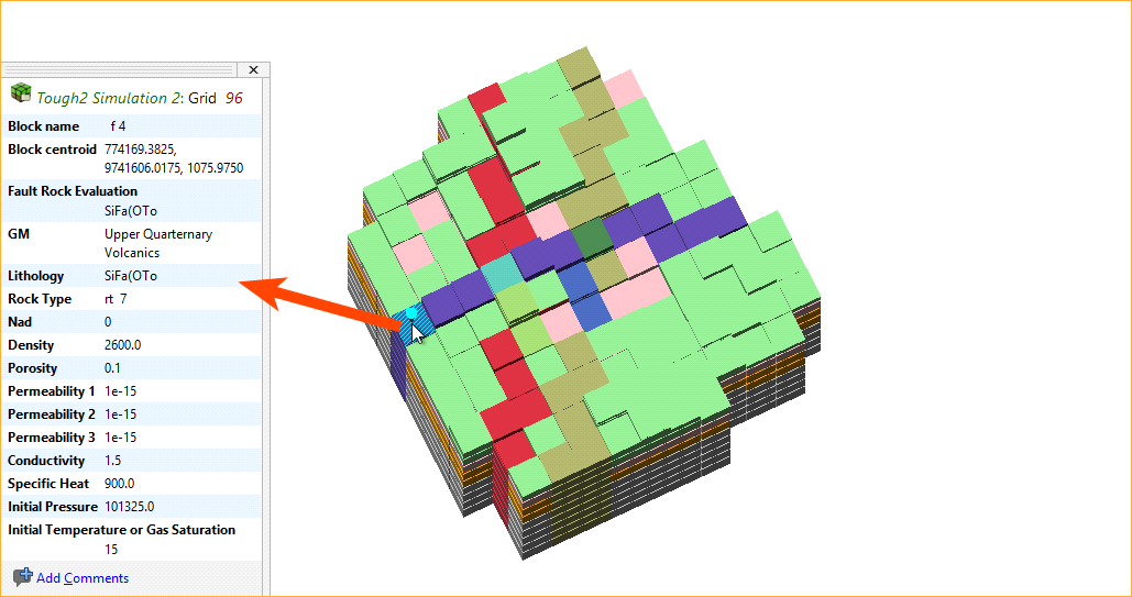
TOUGH2 In-scene Property Display
Clicking TOUGH2 blocks now displays more information about the properties of the selected block:
Vein Reprocessing Improvements
Previously, when a change was made to an interval selection that affected dependent veins, all veins would be reprocessed, including those whose input data had not changed as a result of the interval selection.
Combine Identical Vertices
Meshes in the Meshes folder have a new cleaning option for merging vertices that have the exact same coordinates. This is intended to improve snapping cases where vertices occupy the exact same point in space.
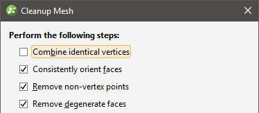
See Cleaning Up a Mesh.
Block Model Export Options
Category Selection on Downhole Points
The New Category Selection tool available on points in the Points folder is now available for downhole points, including LAS points.
Import Meshes From Central
When working on a Central project in Leapfrog Geothermal, you can now import meshes from other Central projects on the same server. This means that it is possible to share up-to-date resources from one project to another improving how multiple users can contribute to a single project. In addition, fast reload functionality allows an up-to-date version of the mesh from the same branch to be easily imported. See Importing Meshes from Central.
View Integration with Leapfrog Geothermal
It has never been so quick and easy to consult a colleague on a tricky model, share impactful visual information with stakeholders or update key personnel on a developing situation.
With a couple of clicks, you can upload a 3D View from Leapfrog Geothermal to the web, where it can be accessed from anywhere in the world. You can set permissions, share and access 3D Views, interrogate the data using slices and rotations and, finally, create ‘slides’ on points of interest in order to focus the conversation.
For complete information on View, visit www.lfview.com.
Leapfrog Geothermal 3.4
- Leapfrog Geo to Leapfrog Geothermal Project Upgrade
- TOUGH2 Flow Simulation Model Improvements
- Isosurfacing of Geophysical Gridded Data
- Import/Export Changes for Geophysical Data
- Assign Selected Intervals to the Base Lithology
- Filtered Wells and Points for Distance Functions
- Option for Section Evaluations to Use Section Extents
- Evaluate Wells onto Curved Sections
- Identify Mesh Parts in the Scene
- Central Projects Organised by Location
- Local Copy Tiles
Leapfrog Geo to Leapfrog Geothermal Project Upgrade
A Leapfrog Geo project can now be upgraded to a Leapfrog Geothermal project. This is a one-way upgrade. See Converting Leapfrog Geo Projects.
TOUGH2 Flow Simulation Model Improvements
A number of minor improvements have been made to Leapfrog Geothermal’s support for the TOUGH2 flow simulator.
- Grid block order. When a TOUGH2 model is export to a .DAT file, the grid blocks are now written out layer-by-layer. Previous versions of Leapfrog Geothermal wrote the grid blocks out in column order.
- Grid block centroids. Grid block centroid x,y,z values are now written to the .DAT file in a format that avoids rounding errors.
- AUTOUGH2 SHORT keyword. AUTOUGH2 input .DAT files containing a “SHORT” section can now be imported into Geothermal 3.4.
- Minimum/maximum display range. Time-dependent data (e.g. pressure, temperature) imported into Leapfrog Geothermal 3.4 from a TOUGH2 listing file will now be displayed with the correct default minimum/maximum value range.
Isosurfacing of Geophysical Gridded Data
Leapfrog Geothermal 3.4 extends support for geophysical data by providing the ability to isosurface geophysical gridded data using an IDW (inverse distance weighted) interpolant model. This creates surfaces and volumes for the specified iso-values. See Inverse Distance Weighted (IDW) Grid Interpolants.
Import/Export Changes for Geophysical Data
The only import/export option available for geophysical point data in the Geophysical Data folder is .csv. Points in .asc, .dxf, .pl3 and .ara formats should be imported into the Points folder.
Assign Selected Intervals to the Base Lithology
When selecting intervals, it is now possible to assign intervals to existing category codes. Previously it was only possible to assign intervals to user-defined codes.
Filtered Wells and Points for Distance Functions
When distance functions are created from wells, points, geophysical points, GIS points and imported GIS lines, it is now possible to filter the object used with any query filter defined for that object.
Option for Section Evaluations to Use Section Extents
When evaluating models or surfaces onto a cross section, an option has been added to allow the evaluation to be limited to the section extents. When selecting objects to evaluate in the Select Model/Surface to Evaluate dialog, the new Clip evaluations to section extents setting is enabled by default.
Evaluate Wells onto Curved Sections
Wells can now be evaluated onto fence sections.
When evaluating wells onto curved sections, a projection is made based on the locations of neighbouring segments of the fence section. This is done by using the bisectors of the angles between each segment and its neighbour to determine the projection point of origin for a given segment of the section. See Adding Styling Wells and Planned Wells.
Identify Mesh Parts in the Scene
When exporting a mesh that has multiple parts, distinguishing between the different parts that can be exported has previously been a case of trial and error. When exporting a single mesh, it is now possible to identify in the scene what parts of a mesh correspond to the select part in the Export Mesh Parts window. See Meshes.
Central Projects Organised by Location
When browsing projects in the Central Projects tab, projects are now grouped by their location tags. The location tags are set in the Admin Portal for a given Central server.
Local Copy Tiles
When viewing a Central project, a list of all local copies is displayed as a series of tiles to help make browsing projects more intuitive. The local copy tile shows the copy’s status and has a link to the history tree and options to delete or publish the project.
Leapfrog Geothermal 3.3
- Terminology Changes
- Central Integration
- Geophysical Data Folder
- Import 2D Points
- Create Mesh From Thickness Values
- Time-Based Visualisation of Geophysical Point Data
- Export Geophysical Grid to CSV
- Graphs
- End Length Control on Numeric Compositing
- Stereonet in 3D
- Two-Way Structural Data Selection
- Improved Statistics on Block Models
- Ignore Duplicate Points
- Improved Copying of Section Layouts
- Batch Export of Serial Section Layouts
- Reload Polylines
- Add Columns to Structural Data, Lineations and Points
- Copying Points and Meshes
- Value Filter for Meshes
- Comments on Subfolders
- Viewing Out-of-Date Objects
- View Geological Models as a Single Object
Terminology Changes
The following changes to naming conventions have been made:
- All references to “borehole” have been replaced with “well”.
- All references to “deep borehole” have been replaced with “well”.
- The Interpolants folder has been renamed and is now the Numeric Models folder.
- Numeric, indicator and multi-domained interpolants are now referred to as “RBF interpolants”, “indicator RBF interpolants” and “multi-domained RBF interpolants”.
Central Integration
Leapfrog Geothermal now operates with Central. See Central Integration for more information.
Geophysical Data Folder
There is a new Geophysical Data folder in the project tree below Polylines and above Structural Modelling. The following geophysical data types can be imported into this folder:
- Magnetotelluric Resistivity (.out WingLink file)
- UBC
- Gocad
- ASEG-DFN
- 2D Grid
- 2D points (csv)
- 3D points (csv)
Some existing functionality has been moved into the Geophysical Data folder:
- The Import Geophysical Points option that was available for the Points folder has been renamed to Import ASEG_DFN and moved into the Geophysical Data folder.
- The Import 2D Grid option is available in the new Geophysical Data folder, as well as from the GIS Data, Maps and Photos folder, where it was originally. If you are importing geophysical data that is in 2D grid format, use the Geophysical Data folder.
- The importation of Gocad, UBC and Magnetotelluric Resistivity models has been moved from the Block Models folder to the Geophysical Data folder.
In addition, you can now import 2D points into the Geophysical Data folder.
Geophysical data that are 3D point data should now be imported into the Geophysical Data folder and not into the Points folder.
Geophysical 3D point data is not checked for duplicates, i.e. duplicate points are allowed.
See the Geophysical Data topic for more information on the functionality available.
Import 2D Points
2D point data can be imported from a csv file into the Geophysical Data folder.
The CSV file contains the following columns:
- Columns 1-2: X,Y
- Columns 3+: Data columns
The elevation can be set to a constant depth or draped onto an existing mesh.
See 2D Points for more information.
Create Mesh From Thickness Values
A mesh can be created from a base mesh and a set of thickness values. The new mesh will have the same X and Y values as the base mesh; only the Z values vary. See Mesh From Thickness Values for more information.
Time-Based Visualisation of Geophysical Point Data
Geophysical 3D point data can be filtered in the scene by another numeric column, e.g. a time or date column. This enables micro-seismic data to be visualised over time. See Visualising Geophysical Point Data for more information.
Export Geophysical Grid to CSV
Geophysical grids in Gocad, UBC and magnetotelluric resistivity (OUT) format can be exported as points to a CSV file. The CSV file will contain:
- X, Y and Z columns, which represent the centre of each grid block
- I, J and K columns, which is the grid block index. I is in the range (1,NI), J is in the range (1,NJ) and K is in the range (1,NK), where NI,NJ,NK are the grid dimensions.
- One or more data columns
See Exporting Geophysical Grids to CSV for more information.
Open Graph on Points
New statistics functionality is now available on points with values. Graphs are available for interval midpoints, grids of points, downhole points, LAS points, imported points and block models.
Note that although the charts displayed can be copied and export from Leapfrog Geothermal, the graphs themselves are not saved when you close the window.
End Length Control on Numeric Compositing
The numeric compositing tools have new options for handling residual segments. It is now possible to add an end-segment to the previous interval, distribute the remainder equally along the hole or within the domain, or discard it, depending on the specified minimum length.
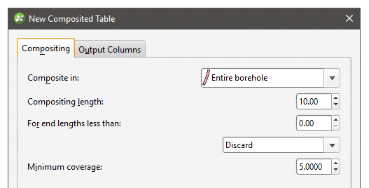
See the Numeric Composites topic for more information.
Stereonet in 3D
Visualise a stereonet in the 3D scene to aid the discovery of trends, relationships and geological structures.
Position the stereonet beside structural measurements, form surfaces and other modelling data to get a different perspective on how the structures relate to the surrounding data. For example, align the view with the intersection of two planes, along the intersection line, to discover potential fold hinges and ore-shoots.
See Displaying the Stereonet in the 3D Scene in the Stereonets topic for more information.
Two-Way Structural Data Selection
When structural data points are displayed and categorised on a stereonet, the data is also displayed in the 3D scene. Structural data can either be selected in the stereonet or in the scene. Initiate a structural selection in the stereonet and continue your selection in the scene. This flexibility maximises the stereonet-scene interaction and optimises structural data analysis.
See Using the Scene Window with the Stereonet in the Stereonets topic for more information.
Improved Statistics on Block Models
Statistics have been improved on block models and sub-blocked models. Multiple interpolant values within each lithology of a geological model can now be compared, and rows can be grouped by category or numeric. Additional statistics such as total volume and coefficient of variation have been included.
See Block Models in the Block Models topic for more information.
Ignore Duplicate Points
When fixing errors on points tables, all duplicates can be quickly ignored using a single-click. This will ignore all but the first row when multiple rows share the same coordinates.
Improved Copying of Section Layouts
The workflow for copying layouts between cross sections has been enhanced to facilitate batch copying of a layout onto multiple cross-sections at once. Layouts were copied by selecting a section and then choosing from the layouts available in the project. Now you choose which layout to copy, then select the sections to copy the layout to. See Copying Section Layouts for more information.
Batch Export of Serial Section Layouts
Export multiple layouts from a serial section. Layouts can either be exported as a single PDF file, or individual PDF, SVG, PNG and GeoTIFF files, which can then be combined into a single zip. See Section Layouts for more information.
Reload Polylines
Polylines created in other Leapfrog projects or software packages can now be reloaded. Latest changes will dynamically update all dependent objects. See Reloading Polylines for more information.
Add Columns to Structural Data, Lineations and Points
Imported points, structural data and lineations can now support importing of new column data. See Importing Planar Structural Data, Importing Lineations and Appending Points Data for more information.
Copying Points and Meshes
Points and meshes may now be copied within the project. This workflow is useful when testing different settings and scenarios.
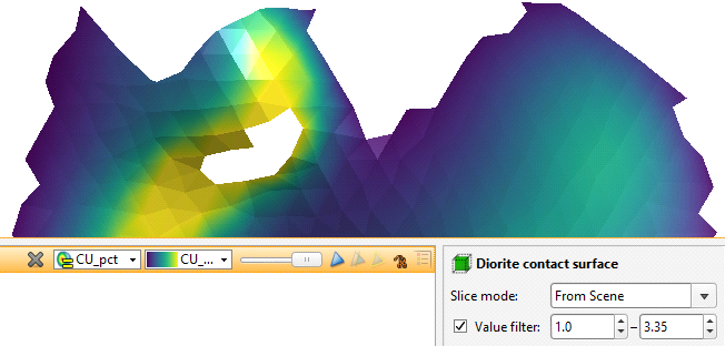
Value Filter for Meshes
Value filters now work with evaluations on meshes, filtering displayed triangles according to the min / max settings. This workflow can be used to focus on an area of interest, for example, to visualise areas such as a steeply dipping slope of a pit wall or a high value area of an interpolant evaluated on a pit-shell or fault plane.
Comments on Subfolders
It is now possible to add comments to subfolders in the project tree:
Viewing Out-of-Date Objects
In previous versions of Leapfrog Geothermal, it has not been possible to view objects in the scene while they are in the processing queue waiting to be processed. It is now possible to view these out-of-date objects while they are queued as these objects will remain in the scene until they start being processed. Out-of-date objects waiting to be processed are displayed in the project tree with their names greyed out.
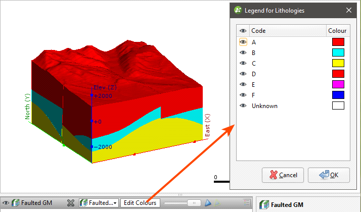
View Geological Models as a Single Object
To improve the organisation of the shape list, geological models now appear as a single object. This makes it easier to work with complex geological models. The visibility of individual volumes is controlled using the Edit Colours option:
Leapfrog Geothermal 3.2
New features and enhancements in Leapfrog Geothermal version 3.2 are:
- Structural Surface
- Form Interpolants
- Stereonets
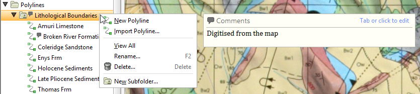
- New Polyline
- Decluster Structural Data
- Linked Surfaces
- Lineations
- Category Selection for Structural Data
- Evaluations on Structural Data
- Set Elevation on Structural Data
- Dip Colouring for Meshes
- Block Model Index Filter
- New Well Evaluations
- Sort Tables by ‘Ignored’ Flag
- Show Mesh Border
- Copy Polyline
- More Inputs for Structural Trends
- New Volume Generation Options
- Moving Plane Handles
- Curved Fence Sections
- Textured .OBJ Meshes
- Well Correlation Improvements
Structural Surface
The structural surface is a new method for building geologic contact surfaces within a geological model. As well as standard surface input data, structural surfaces can use non-contacting structural data to influence and guide the overall geometry. Bedding data from pit face-mapping, downhole measurements and surface mapping can be combined together with drilling lithology contact data and surface contact mapping.
To learn more, see the Structural Surfaces topic.
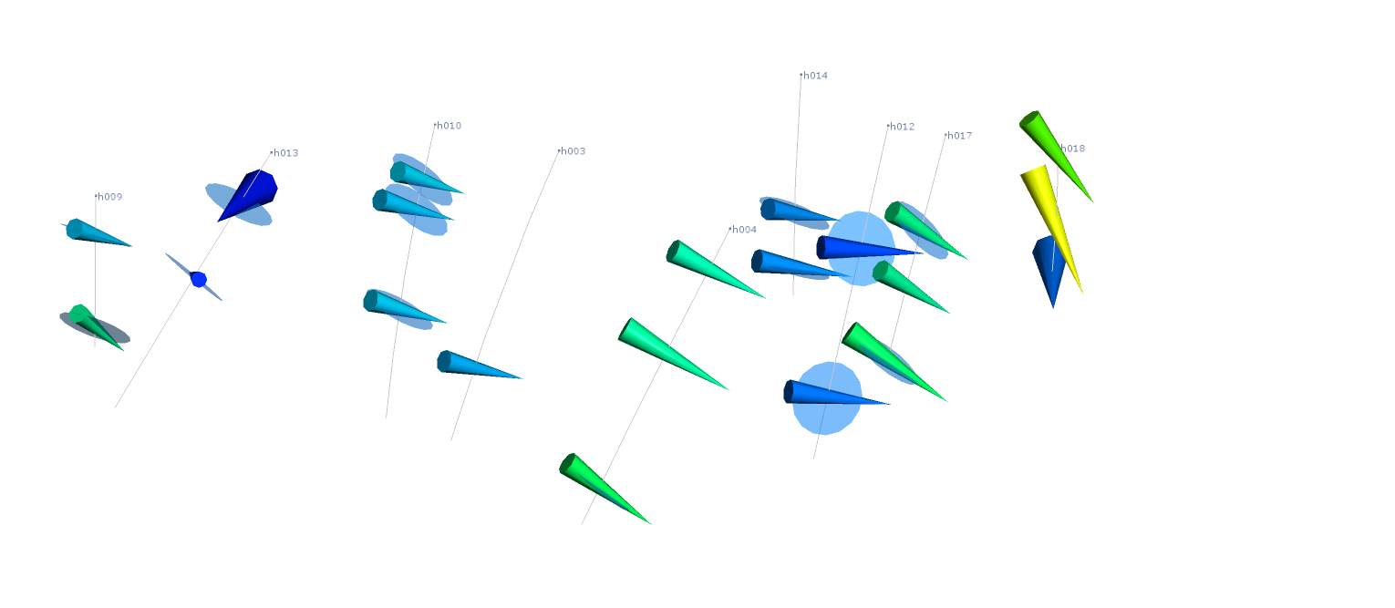
Form Interpolants
Structural form interpolants combine bedding or foliation orientation data from pit face-mapping, downhole measurements and surface mapping to interpolate and visualise the form of the rock fabric of a region. Form interpolants may be visualised as isosurfaces or evaluated onto surfaces, points and block models. Isosurfaces of form interpolants may be dynamically applied to structural trends to control the anisotropy of grade models.
To learn more, see the Form Interpolants topic.
Stereonets
Leapfrog Geothermal now includes an interactive stereonet tool, providing the capability to interpret complex structural data sets through stereographic projection. Stereonets can be saved as part of a Leapfrog Geothermal project for quick recall, supporting any combination of mapped, downhole or declustered structural data.
Several built-in visualisation options such as contouring and statistics provide the means to discover hidden trends, relationships and geological structures. An interactive selection and categorisation workflow makes it easy to classify distinct populations of measurements. The selected regions and colourings are simultaneously linked with the 3D scene for a wider perspective. Stereonet plots can be exported in PDF format.
To learn more, see the Stereonets topic.
New Polyline
This powerful new drawing tool supersedes the previous straight-segment and 2D-curved line types. The new polyline is a unified editing and interpretation tool, supporting full 3D drawing modes for curved and straight lines, as well as single points. The new tool has options to control the pitch of surfaces by adjusting a line’s ribbon orientation, or adding points with normals. Simple 2D lines can be drawn on the slice plane, and 3D curves can be drawn on any in-scene objects, such as topographic surfaces and drillhole contacts.
The new drawing tool is available anywhere linework is able to be drawn in a project. Also new to this version are refreshed custom line editors for GIS lines, vein boundaries and direct surface edits. New import and export formats mean the new polyline is natively compatible with Leapfrog Mining as well as supporting smooth drag-and-drop transfer into Leapfrog projects.
To learn more, see Drawing in the Scene.
Decluster Structural Data
Leapfrog Geothermal now easily handles large, complex structural datasets with the help of a powerful declustering tool. Any planar structural dataset may be thinned to manageable sizes using the new declustering tool, which retains representative samples across the dataset based on range and angle tolerance parameters.
To learn more, see Declustering Planar Structural Data in the Structural Data topic.
Linked Surfaces
Any existing surface can now be used as an input to another model within the same project. Complex geology often requires complex modelling solutions, making it necessary to build a key surface in one model, then include it in another. Take a dike-swarm for example; when it post-dates a fault, dynamically linked surfaces mean an unfaulted model can be created for the complex dykes then combined with the faulted geology to produce a cohesive model that honours the geological history.
Lineations
Measured linear structural features can now be imported and visualised. View, select, and categorise lineations in both the stereonet plot and the 3D scene. Use these to guide your interpretations with a better understanding of the regional deformation.
To learn more, see Importing Lineations in the Structural Data topic.
Category Selection for Structural Data
The familiar brush-selection tool is now available for both planar and linear structural data. This facilitates a simple and powerful workflow of quickly categorising data to aid interpretation or guide downstream modelling. The category selection tool can be used to quickly ignore a large selection of measurements, especially when combined with the ability to evaluate models on structural data.
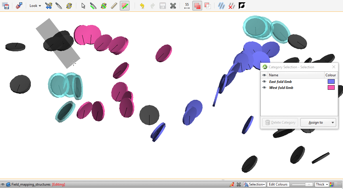
To learn more, see Assigning Structural Data to Categories in the Structural Data topic.
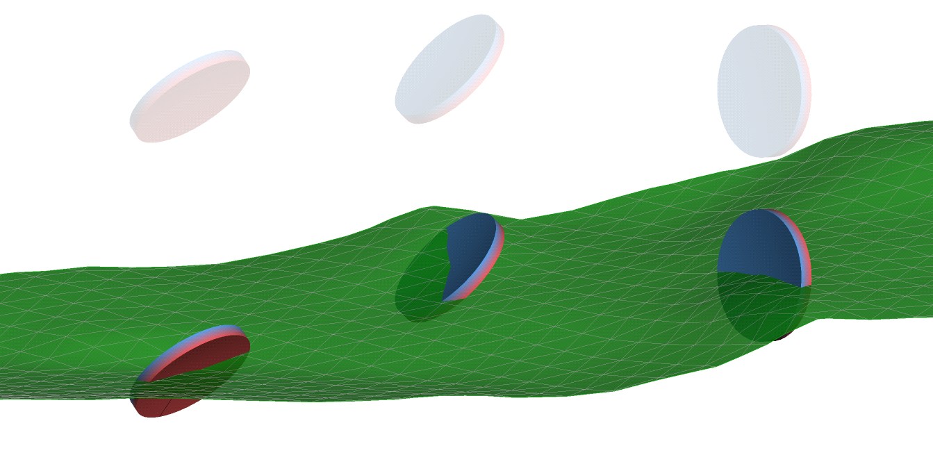
Evaluations on Structural Data
Geological models or grade interpolants can now be evaluated on planar and linear structural data, allowing them to be visually filtered by volumes of geological models. Interpolant evaluations enable a workflow to identify the orientations that are associated with high grade mineralisation.
Set Elevation on Structural Data
Structural data can now be projected vertically onto any surface, such as your topography. Sometimes when surface mapping structural data, the elevation measurements are inaccurate or inconsistent, but now this workflow provides a way to repair it.
To learn more, see Setting Elevation for Structural Data in the Structural Data topic.
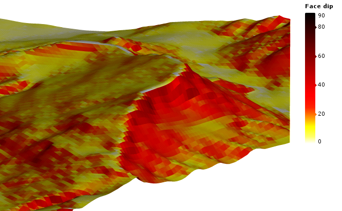
Dip Colouring for Meshes
All surfaces and meshes can be coloured by the dip-angle of the triangle faces. This allows you to easily identify steeply dipping areas or flat spots.
Block Model Index Filter
New index filters create a rapid way of visualising 3D slices and sub-units in block models. Index filters support modes and are available for blocked, sub-blocked and geophysical models.
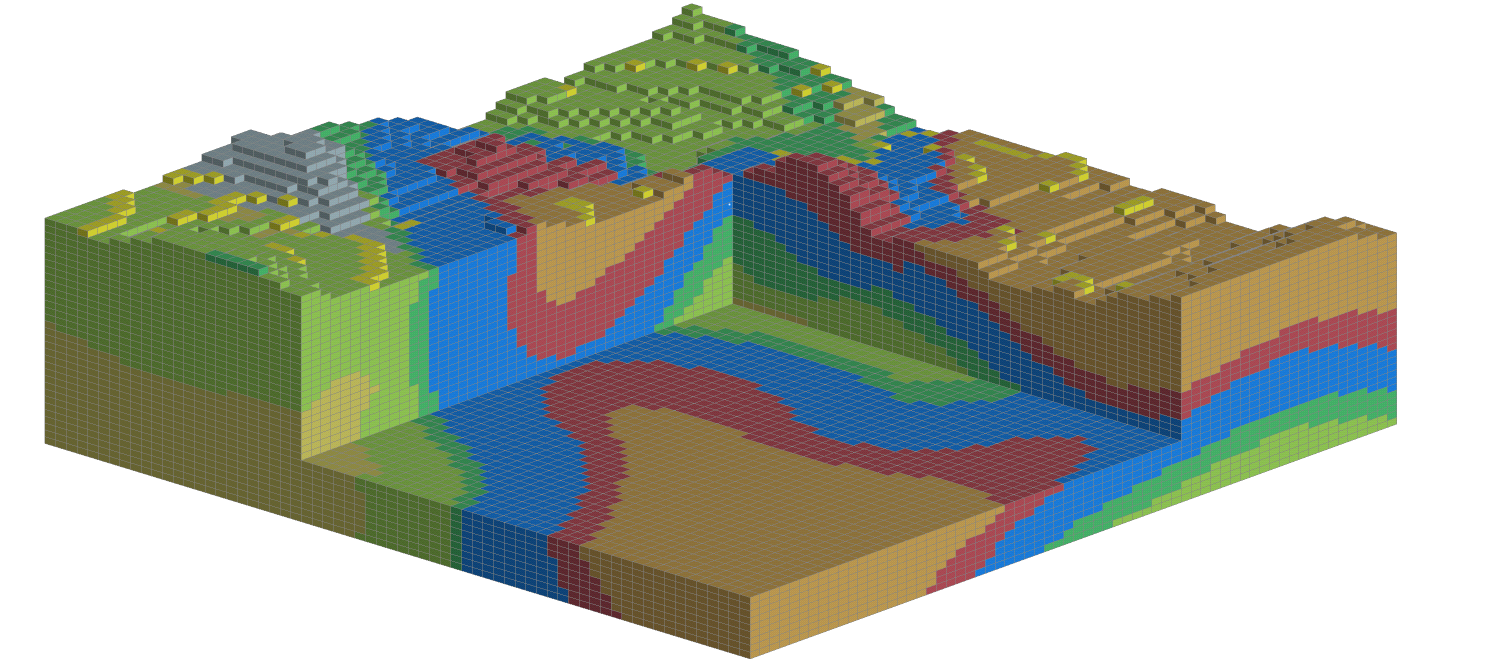
New Well Evaluations
When evaluating (backflagging) geological models onto wells, you can now choose to evaluate the faulted output volumes or fault blocks. This allows additional numeric compositing workflows where you can composite within each separate domain in a geological model.
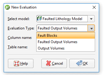
To learn more, see the Back-Flagging Well Data topic.
Sort Tables by ‘Ignored’ Flag
Tables in Leapfrog Geothermal (points, drilling, structural etc.) may now be re-ordered by rows that have been ignored. This enables a quick way to find all ignored rows and make batch changes.
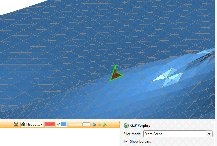
Show Mesh Border
You can now show the border for all imported or extracted meshes which are not closed volumes. This helps to diagnose problematic meshes by identifying any areas where the mesh is open.
Copy Polyline
Individual polylines can now be copied within the project. Being able to easily copy polylines provides a rapid workflow for testing multiple interpretations.
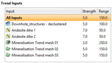
More Inputs for Structural Trends
Structural trends can now be derived directly from planar structural data. You can also apply any mesh in the project, allowing you to dynamically link your mineralisation structural trend to your fault and contact surfaces.
New Volume Generation Options
New volume generation modes for geological models provide the flexibility to control the way the implicit modeller creates volumes from contact surfaces and faults. The three modes for volume generation make it possible to balance triangle alignment with processing performance.
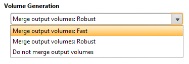
To learn more, see Volume Generation Options in the Editing a Geological Model topic.
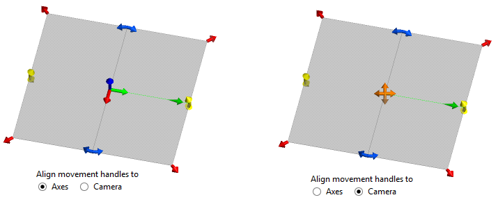
Moving Plane Handles
The moving plane tool can now be moved either in the direction of the axes or relative to the current camera view.
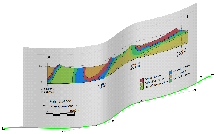
Curved Fence Sections
Fence sections now support curves generated by the new polyline tool. This can be useful for generating sections that follow a decline tunnel as it curves underground, for example.
Textured .OBJ Meshes
Wavefront Obj format is an open format geometry format widely supported by 3D graphics applications. Leapfrog Geothermal now supports importing OBJ meshes with textures, which broadens Leapfrog’s ability to import mine scan meshes like pit faces, stopes and tunnels.
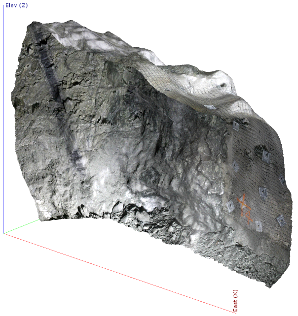
To learn more, see Meshes with Textures in the Importing a Mesh topic.
Well Correlation Improvements
Numeric columns from both points and intervals can now be displayed as bars, lines or points in the 2D well correlation tool. This allows for consistent numeric display standards regardless of the data type.

To learn more, see the Well Correlation Tool topic.
Leapfrog Geothermal 3.1
- Create Guide Points
- Import LAS Points
- Categorise Points and Collars in the Scene
- Batch Importing and Reloading GIS Data
- Extended Multicore Processing
Create Guide Points
Guide points can now be created from any category data in the project and added to surfaces. Category data that can be used to create guide points includes downhole category data, LAS points, category data on imported points and interval midpoints. See Creating Guide Points for more information.
Import LAS Points
LAS 1.2 and 2 well logs can now be imported into Leapfrog Geothermal. This import workflow can handle multiple LAS files and will convert them into a single well points table. Imported LAS files can be viewed in 3D as a single object, and columns of data common across all LAS files can easily be used as input into an RBF interpolant. Query filters are automatically created on import for each of the original LAS files, making it easy to see each of the individual files. See Importing LAS Points Down Wells for more information.
LAS files are ideal data to view in the well correlation tool.
Categorise Points and Collars in the Scene
It is now possible to sort points and collars into categories. This works in a similar manner to the interval selection tool: The points are added to the scene and then manually selected and assigned to categories. See Categorising Points for more information.
Batch Importing and Reloading GIS Data
Imported ESRI Geodatabases and MapInfo batch files are now added to the project tree as part of a parent object. This makes it clear whether individual GIS objects came in on their own or as part of an import from a Geodatabase or MapInfo batch import. These GIS collections can also be reloaded.
Extended Multicore Processing
In 2014, Leapfrog introduced the ability to use up to 4 cores when processing. Leapfrog Geothermal 3.1 increases this capability to 8 cores. Those with high end computers with 8-core processors can now access all of their computer’s power to significantly reduce processing times when tackling complex modelling problems.
Leapfrog Geothermal 3.0
- Well Correlation Tool
- Interpretation Tables
- Offset Mesh in Geological Models
- Stratigraphic Sequence Improvements
- UBC Grids
- Colour Gradients
- Cross Section Layouts
- Subfolders
- Improved Project Tree Controls
- GIS Visibility in the Project Tree
- Improved Tabbed Interface
- Exact Mesh Clipping
- Add Contour Polylines to Indicator Interpolants
- Reload GIS Data
- Set Background Lithology
- Set Elevation of Points
- GIS Line from Mesh Intersections
- Fast Copy for Geological Models
- Add Interval Mid-points to Surfaces
- Unshare Polylines
Well Correlation Tool
The new well correlation tool is a ‘Leapfrog take’ on a very common workflow across many deposit-styles. Quickly select and view wells and other required data. Rearrange wells and data columns, and zoom and scroll with intuitive controls. Save and share templates and styles across projects.
To learn more, see the Well Correlation Tool help topic.
Interpretation Tables
Being able to view and compare data is only half the story. Leapfrog Geothermal 3.0 introduces a new way of working with well data: the interpretation table. Open a table and move the start and end of intervals, re-assign intervals and create brand new intervals. Rapidly compare previous logging to other measurements (assays, geochemistry and geophysics) and re-interpret.
To learn more, see Interpretation Tables in the Well Correlation Tool help topic.
Offset Mesh in Geological Models
The new Offset Surface Tool is useful for modelling stratigraphic deposits where surfaces share a common deformation history and have a similar overall shape. Define and constrain the reference mesh from a particularly well-drilled area and, therefore, constrained unit. Alternatively, define the reference mesh using any other input option such as polylines, structural data and structural trends. Constrain the thickness of the volumes with minimum/maximum offset or a fixed offset distance.
To learn more, see the Offset Surfaces help topic.
Stratigraphic Sequence Improvements
Reduce the number of polyline edits needed. Constrain stratigraphic sequence surfaces using well intervals and contact points.
To learn more about using stratigraphic sequences, see the help topic.
UBC Grids
Import UBC geophysical grids for evaluation of geological and interpolant models. Export and evaluate in UBC format. Enable the visualisation of geophysical models alongside drilling and models. Use the workflow to make constrained inversions directly from Leapfrog geological models.
To learn more, see the UBC Grids help topic.
Colour Gradients
Enhance data visualisation with colour gradient import and export. Import colour gradients from various GIS or geophysics packages (.tbl, .clr & .lut).
To learn more, see Numeric Data Colourmaps in the Visualising Data help topic.
Cross Section Layouts
- Display assay data as bar and line graphs in section layouts.
- Evaluate block models on cross sections and add to section layouts. Includes sub-blocked, MODFLOW, FEFLOW and UBC models.
- Display sections in the 3D scene.
- Export section layouts as GeoTIFFs.
To learn more, see the Section Layouts help topic.
Subfolders
Create subfolders to sort and file objects in projects.
To learn more, see Subfolders in The Project Tree.
Improved Project Tree Controls
Display lines in the project tree to better show relationships. In the Settings window, click on User Interface and enable Show Tree Lines.
More options enable rapid opening or closing of folders. Collapse the entire project by right-clicking on the top of the project tree and selecting Collapse All. Hotkeys for opening and closing folders include:
- Ctrl + shift + left arrow collapses all folders.
- Right arrow expands a collapsed folder or object but keeps child objects collapsed.
- Shift + right arrow expands a collapsed folder or object and child objects.
- Left arrow collapses an expanded folder or object but keeps child objects expanded.
- Shift + left arrow collapses an expanded folder or object and child objects.
Hotkeys work with more than one object selected.
GIS Visibility in the Project Tree
A copy of all GIS data is created on import and projected on the topography. This projected copy is now visible in the project tree underneath the topography object.
Improved Tabbed Interface
In order to improve the way large dialogs interact with the scene view, there are new options in the project Settings window. You can choose whether tabbed dialogs open to the main window, a separate window or where the last tab was moved to. This improvement has been applied to well tables, section layouts, image georeferencing, movie editing and image rendering.
Exact Mesh Clipping
Switch on exact clipping for meshes, removing tags that overhang the clipping mesh.
For more information, see:
- Surface Generation Options in the Editing a Geological Model help topic
- Output Settings for an RBF Interpolant in the RBF Interpolants help topic
- Output Options in the Multi-Domained RBF Interpolants help topic
- Indicator RBF Interpolant Surfacing and Volume Options in the Indicator RBF Interpolants help topic
Add Contour Polylines to Indicator Interpolants
Adjust indicator interpolants using contour polylines, similar to how contour polylines are used with RBF interpolants. Instead of selecting a specific value, use 0 (outside), 1 (inside) or the isosurface value.
To learn more, see Adding a Contour Polyline in the Indicator RBF Interpolants help topic.
Reload GIS Data
Reload GIS data to reflect changes during the project life-cycle. Automatically re-run and update dependant surfaces and models.
To learn more, see the Reloading GIS Data help topic.
Set Background Lithology
Set one of the lithologies as the background lithology for geological models and fault blocks. This is an alternative to using the “Unknown” lithology and is useful for faulted models.
Set Elevation of Points
Project onto a surface and overwrite the elevation/z value for points. Set the elevation of points that don’t project onto the surface.
To learn more, see the Setting Elevation for Points help topic.
GIS Line from Mesh Intersections
Create a new GIS line from two intersecting meshes. Use this for visualisation or as an input into Leapfrog models.
To learn more, see Creating a New GIS Line from Intersecting Meshes in the Creating a New GIS Line help topic.
Fast Copy for Geological Models
Rapidly copy the geological model for easier scenario testing.
Add Interval Mid-points to Surfaces
Use extracted mid-points in the Points folder as inputs for surfaces.
Unshare Polylines
Create a local copy of any polyline when it is no longer correct or useful to share the same polyline.
To learn more, see The Project Tree in The Project Tree.
Got a question? Visit the My Leapfrog forums at https://forum.leapfrog3d.com/c/open-forum or technical support at http://www.leapfrog3d.com/contact/support