Model Targets (Batch)

Use the Model Targets (Batch) option (Geosoft.uxo.gxnet.dll(Geosoft.GX.UXO.UceTargetFit;Run)*) to model/invert your targets from total field magnetic data or Geonics EM61 data using either simple square anomaly windows or more complex polygon anomaly windows.

Expand to see the locations (menus) where this option is available.

Model Targets (Batch) dialog options

Target Database
Name	Specify your target database: enter or select the database name from the list of databases added to your project. You can also browse and select a database file from a different location. At the onset, the target database must contain the four channels: X and Y, which define where your targets are located, an ID and a Mask channel. On output, it is populated with the modelled results for each target location. See the Application Notes below for more information. Script Parameter: UXANALYZE.TARGETGDB
Group	Select the target database group to model from the dropdown list. Script Parameter: UXANALYZE.TARGETGRP
ID channel	Select the target ID channel from the list of database channels. Script Parameter: UXANALYZE.TARGETID
Mask channel	Select the target database mask channel to filter out specific targets. Only the targets with a mask (channel value) of 1 will be processed. If the value is set to 0 or dummy (*), the corresponding target will be ignored. If the field is left blank, no mask will be applied. Script Parameter: UXANALYZE.TARGETMASK
Survey Database
Name	Specify the database containing your survey X, Y, and data channels: enter or select the database name from the list of databases added to your project. You can also browse and choose the database file from a different location. Script Parameter: UXANALYZE.INPGDB
Altitude channel	Select the altitude channel if present in the survey database. Otherwise, the Instrument height above ground entry under the General Parameters section will be used. Script Parameter: UXANALYZE.ALTCHAN
Instrument type: Magnetometer
Mag channel	If "Magnetometers" is selected as the instrument type under the General Parameters section, the Mag channel field will appear. From the dropdown list, select the data channel in the survey database that contains the magnetic data to be modelled. This is a mandatory field. Script Parameter: UXANALYZE.SENCHAN1
Instrument type: EM-61
Upper channel	If "EM-61" is selected as the instrument type under the General Parameters section, the Upper channel field will appear. From the dropdown list, select the upper data channel from the survey database. Script Parameter: UXANALYZE.SENSCHAN1
Lower channel	If "EM-61" is selected as the instrument type under the General Parameters section, the Lower channel field will appear. From the dropdown list, select the lower data channel from the survey database. Script Parameter: UXANALYZE.SENSCHAN2
Instrument type: EM-61 Mark-II
Time gate 1	If the "EM-61 Mark II" type is selected under the General Parameters section, four time gate channels will appear. Time gate 1 ("Mode 4")/Time gate T ("Mode D") is the upper channel. For further detailed explanation of the Modes please refer to the Geonics manual. Script Parameter: UXANALYZE. SENSCHAN1
Time gate 2	Select the first lower time gate. Script Parameter: UXANALYZE. SENSCHAN2
Time gate 3	Select the second lower time gate. Script Parameter: UXANALYZE. SENSCHAN3
Time gate 4	Select the third lower time gate. Script Parameter: UXANALYZE. SENSCHAN4
General Parameters
Instrument type	Select the type of instrument from the dropdown list. Depending on your selection, different fields will be displayed in the Survey Database section (as per above). Script Parameter: UXANALYZE.INST
Instrument height above ground	Specify the height of the instrument above ground. This is only required if the survey database does not contain an altitude (elevation) channel. Script Parameter: UXANALYZE.COILHEIGHT
Polygon directory	If you have created polygons to delineate target extents, the polygon files will be saved in the workspace subdirectory (_wrk\plys) of your current project. The location of these target polygons will be displayed by default in this entry. If you want to use other polygons, or if the entry is empty, click the browse button to specify the location of the target polygons. If your selected polygon directory does not contain polygon files, an error will be prompted at the end of the process. The generated log file "<TargetDatabase>_Modelling_Error.log" will capture the IDs of the targets that are missing in a window polygon (PLY) file. In this case, square windows of the target sizes will be generated and used for modelling. Script Parameter: UXANALYZE.DIRECTORY
Polygon prefix	With a polygon directory located, the tool will scan the list of targets in the specified location and will provide you with a list of polygon prefixes to choose from. The polygon (PLY) file name convention is " Prefix_TargetGroup_TargetID". If there are no entries, enter a target polygon prefix. It is recommended to incorporate the window size or another identifying feature in the prefix. Script Parameter: UXANALYZE.PREFIX
Target window size	If there are no polygon files available, square windows can be defined and created by specifying the target window size. Also, if a target is found with no polygon associated with, a square polygon of the target size will be generated and used for modelling. The log file "<TargetDatabase>_Modelling_Error.log" will record the target ID that is missing a window polygon (PLY) file. Script Parameter: UXANALYZE.ANOMALY
Sensor Specific Parameters
Instrument type: Magnetometer
Date (YYY/MM/DD)	Specify the approximate survey date using the format yyyy/mm/dd. Default is the value of the flight date from the survey database. This date is to select the IGRF model year. Script Parameter: none, only used when interactive
[Recalc]	Click on the Recalc button to calculate the geomagnetic reference field (GRF). The GRF is determined based on the location of the survey and the entered date. Your survey must have a coordinate system set, (i.e., not be unknown); if it is not set, you will be prompted to set a coordinate system.
Total field	Specify the total field value. Script Parameter: UXANALYZE.FIELDSTRENGTH1
Inclination	Specify the inclination value. Script Parameter: UXANALYZE.INCLINATION1
Declination	Specify the declination value. Script Parameter: UXANALYZE.DECLINATION1
Instrument type: EM-61
Instrument coil separation	Specify the coil separation between the upper and lower coils. Script Parameter: UXANALYZE.COILHEIGHT1
Instrument type: EM-61 Mark-II
Instrument coil separation	Specify the coil separation between the upper and lower coils. Script Parameter: UXANALYZE.COILHEIGHT1
Mode	Select either Mode D (Differential) or Mode 4 (4 time-gate). Default selection is D. Script Parameter: UXANALYZE.MODE

Application Notes

For each target in your target database, the magnetic data or Geonics EM61 data is extracted and modelled/inverted to determine a potential source location and parameters. To use the Model Targets (Batch) option to invert your data, select the sensor type and enter the required parameters. At the end of the process, the target database is populated with the inverted or modelled parameters.

If an error happens during the batch process, the error messages are logged in a file named "<TargetDatabase>_Modelling_Error.log".

Anomaly Window Polygons

For each target, a polygon window of data about the target location is extracted and modeled. The window should be large enough to encompass a single anomaly along with some background data but should exclude adjacent anomalies. These polygon windows can be defined in two ways:

As a simple square of the size - defined in the target window size parameter.
As a polygon - created by either Calculate Signal Strength, Signal to Noise Ratio and Size or Display Target Windows and edited as needed using Redefine Target Windows .

The polygon files are expected to be in the polygon directory (default is "_wrk\plys"), with names that have the form "<Prefix><Target Database><Target Group><Target ID>.ply". When the data is modelled, polygons of simple square windows are automatically generated and stored in the polygon directory; these will have the suffix "sqwin" and are used to extract the initial data-chip. The square data-chip is then further refined using the (complex) polygons you provide. If a polygon cannot be found for a target, the square window will be used for modelling, and a warning will be placed in the modelling log file.

When working with your polygon using Display Target Windows and Redefine Target Windows, on your map, you should also display your line path or survey locations. The modelling is based on the location of the measured data, so across survey lines you may need to extend the polygon to the next adjacent survey line to have ‘background’ data included.

Inversion Results

Magnetic Parameters

The inversion of the magnetic data will return the following source parameters in your target database:

Fit_error: Inversion error flag:
* - Unable to locate target is survey the database
0 - No error
1 - Anomaly not strong enough to fit
2 - Not enough data points selected for modelling
3 - Zero RMS noise
-3 - Maximum number of iterations reached
4 - Memory allocation error for target
5 - Square root of negative number encountered when fitting target
6 - Division by zero
7 - Matrix inversion problem
8 - Parameter values changed too much relative to initial estimates
9 - Fit process did not converge
Fit_coh: The model coherence, a measure of how well the modelled data fits the measured or observed data; specifically, the correlation coefficient squared (dimensionless). A high fit coherence does not guarantee that the fit results are accurate – only that the match between modelled and measured data is high. Multiple solutions may exist. The fit quality also depends on the number of data samples being passed to the fitting algorithm. The fewer the samples the easier it is to get a high fit coherence.
Fit_ModErr: The model error, a measure of the error in the modelled data (percent). This is calculated by sqrt(1-correlation coefficient squared) *100.
Fit_depth: The depth of the source dipole from the surface (survey distance units)
Fit_x: The X location of the source dipole (survey distance units)
Fit_y: The Y location of the source dipole (survey distance units)
Fit_dec: The declination of the source dipole (degrees)
Fit_inc: The inclination of the source dipole (degrees)
Fit_MagneticMoment: magnetic dipole moment, a measure of the magnetic source (Amp-m2)
Fit_size: Empirically calculated diameter of the object (distance units). The size estimate output from the magnetic data is a function of the object orientation with respect to the earth’s field. The standard deviation of the size estimate is approximately 30% of the ordnance diameter. The apparent size is inferred from the radius of steel sphere, which has the same magnetic dipole as the target. In general, the size output from magnetic data is more robust than the size using EM data for common targets. The “fit_size” parameter should be used as a relative indicator of size and not as an absolute indicator of UXO caliber.
Fit_Solid angle: The angle between the earth's magnetic field and the inverted source dipole (degrees).
Index2SubsetGDB: The group number in the modelling or subset database holding the corresponding data.
Comments: Initially this string is of zero length - you may populate it with target related information.

EM61 Parameters

The inversion of the EM61 data will return the following source parameters in your target database:

Fit_error: Inversion error flag:
* - Unable to locate target is survey the database
0 - No error
1 - Anomaly not strong enough to fit
2 - Not enough data points selected for modelling
3 - Zero RMS noise
-3 - Reached maximum number of iterations
4 - Memory allocation error for target
5 - Square root of negative number encountered when fitting target
6 - Division by zero
7 - Matrix inversion problem
8 - Parameter values changed too much relative to initial estimates
9 - Fit process did not converge
Fit_coh: The model coherence, a measure of how well the modelled data fits the measured or observed data; specifically, the correlation coefficient squared (dimensionless). Ideally, a fit coefficient of 0.995 or greater is desired for EM data to have confidence in the shape information (expressed by the polarizabilities (“betas”) – see definition below). However, if only size and depth are of interest, then a lower fit coherence (i.e. ~0.98) may be acceptable. A high fit coherence does not guarantee that the fit results are accurate – only that the match between modelled and measured data is high. Multiple solutions may exist. The fit quality also depends on the number of data samples being passed to the fitting algorithm. The fewer the samples the easier it is to get a high fit coherence (dimensionless).
Fit_ModErr: The model error, a measure of the error in the modelled data (percent). This is calculated by sqrt(1-correlation coefficient squared) *100.
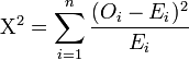
Fit_chi2: The Chi-Square Statistic is a measure of the error in the model data (dimensionless). It is calculated across the full-time decay for each Transmitter and Receiver combination as ∑((y-yfit)/sdev)2.
The value of the Chi Square test-statistic is:
Where:
= Pearson's cumulative test statistic, which asymptotically approaches a distribution.
= observed or measured data
= expected or modelled data
= the number of valid time gates
Fit_depth: The depth of the source from the surface (survey distance units)
Fit_x: The X location of the source (survey distance units)
Fit_y: The Y location of the source (survey distance units)
Fit_theta: Inclination of the source dipole (degrees)
Fit_phi: Declination of the source dipole (degrees)
Fit_psi: Rotation of the source dipole (degrees)
Fit_b1, b2, b3: The three polarizabilities or response coefficients (“betas”) that represent the eigenvalues of the magnetic polarizability tensor. The relative size of the coefficients provides information about the shape of the object. For cylindrical, metallic, and isolated objects, we expect b1>b2≈b3. For spherical objects, b1≈b2≈b3. They can be thought of as components along the three orthogonal axes of the induced dipole.
ModelingChannels: In the case of EM61MKII the channels used to derive the modelled parameters. Note that if multiple channels are modelled, multiple sets of modelled parameters will result. The later source parameters are appended to the bottom of the target group.
Index2SubsetGDB: The group number in the modelling or subset database holding the corresponding data.
Comments: Initially, this string is of zero length - the user may populate it with target related information.

Modelling Database

For fast access, the process sorts the survey data by X then Y into one big bin. Then for each target, it extracts a window of data centered on the target and of the specified window size. This data is saved in a modelling or subset database as:

<SurveyDatabase>_<TargetDatabase>_<TargetGroup>.gdb

For each target, the extracted data is saved in a random group by Target ID number. In addition to this window, the profile line closest to the target is also extracted. All the data that lies within a square window (target window size) is extracted into a channel with the same name as your original data channel. This is then refined using the polygon anomaly window (if existing) and saved into a channel with the suffix "_final". The model is then calculated, and the resulting data is saved into a channel with the suffix "_model". The residual – the difference between the observed and model data is also calculated and saved into a channel with the suffix "_residual".

This tool is developed in partnership with Acorn Science and Innovation (AcornSI).

*The GX tool will search in the "gx" folder. The GX.Net tools, however, are embedded in the Geosoft.uxo.gxnet.dll located in the bin folder. If running this GX interactively, bypassing the menu, first change the folder to point to the bin folder, then supply the GX.Net tool in the specified format.