
Drilling Data
Drilling data forms the basis for creating models in Leapfrog Works. Import drilling data by right-clicking on the Borehole Data folder and selecting one of the import options:
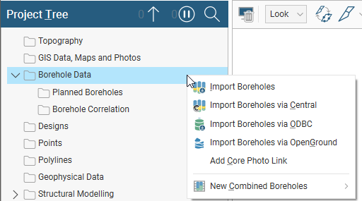
Each of these options is discussed in the Importing Drilling Data topic.
Because drilling data often contains errors that reduce the reliability of a model, Leapfrog Works has tools that help you to identify and correct errors and work with the data. These tools are described in the Identifying and Correcting Data Errors in Leapfrog Works topic.
Once imported and corrected, drilling data usually requires further processing before any models are built. Leapfrog Works has a number of tools for processing drilling data; some of these options add new columns to existing tables and some create new tables.
Options that add new columns to existing tables are:
- Selecting Intervals. If the lithologies in a column are poorly sorted, you can display the column in the scene and use the interval selection tool to work with all the segments and sort them into new units.
- Splitting Lithologies. Lithology units may be incorrectly grouped, which can become apparent when you display boreholes in the scene. The split lithologies tool lets you create new units by selecting from intervals displayed in the scene.
- Grouping Lithologies. The group lithologies tool lets you define a new unit to which existing units are added. For example, a sandstone deposit might appear in an interval table as poorly-sorted and well-sorted units. The group lithologies tool lets you group both units into a single sandstone unit.
- Overlaid Lithology Column. You may have two versions of an interval column, one that contains draft data and one that contains the final version. The final version may contain gaps, which can be filled in using the draft version. The overlaid lithology tool lets you combine the two columns to create a new column.
- Category Column From Numeric Data. When you have numeric data you wish to use with the lithology and category modelling tools, you can convert the numeric data to a category column.
-
Evaluated Columns. An evaluated column adds data to a table from another source within the project, often integrating some information generated from your analysis activities back onto some source data tables (back-flagging).
- Majority Category From Other Table. When you have category data such as economic compositing status or lithology data from another table, you can back-flag it onto an interval table.
Options that create new tables are:
- Category Composites. Sometimes unit boundaries are poorly defined, with fragments of other lithologies within the lithology of interest. This can result in very small segments near the edges of the lithology of interest. Modelling the fine detail is not always necessary, and so compositing can be used to smooth these boundaries.
- Majority Composites. Category data can be composited into interval lengths from another table or into fixed interval lengths. The compositing is based on a majority percentage where each interval is assigned a category based on the category that makes up the highest percentage of the new interval.
- Numeric Composites. Compositing numeric data takes unevenly-spaced drilling data and turns it into regularly-spaced data, which is then interpolated. Numeric data can be composited along the entire borehole or in selected regions. You can also set the compositing length from the base interval table.
- Back-Flagging Drilling Data. Evaluating geological models on boreholes creates a new lithology table containing the lithologies from the selected model.
- Merging Drilling Data Tables. If you are working with columns in different interval tables in the same drilling data set, you can create a new merged table that includes columns from these different tables. Columns created in Leapfrog Works can be included in a merged table.
Finally, when you have data across multiple drilling data sets that you wish to use elsewhere in the project, you can create a combined drilling data set that contains interval values, downhole points, downhole structural data and screens data from other drilling data sets. See Combining Drilling Data Sets.
The rest of this topic discusses:
- How Drilling Data is Organised in Leapfrog Works
- Displaying Drilling Data
- Viewing Drilling Data Table Statistics
- Exporting Drilling Data
How Drilling Data is Organised in Leapfrog Works
In Leapfrog Works, drilling data is organised into drilling data sets, which are made up of a collar file, a survey file and at least one interval table. A drilling data set can also contain:
- Downhole points
- LAS points
- Downhole planar structural data
Previous versions of Leapfrog Works supported just one drilling data set, but in Leapfrog Works 2021.1 forward, multiple drilling data sets can be imported.
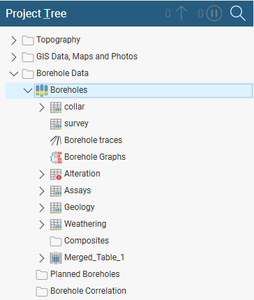
Here, a single drilling data set made up of a number of tables has been added to the project, stored in the Borehole Data folder:
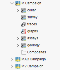
Here there are three drilling data sets, M Campaign, MAC Campaign and MV Campaign:
You can open each table (![]() ) in a drilling data set by double-clicking on it. The table will be displayed and you can make changes in it, as described in the Working With Data Tables topic. When there are errors in the data, the relevant table will be marked with a red exclamation mark (
) in a drilling data set by double-clicking on it. The table will be displayed and you can make changes in it, as described in the Working With Data Tables topic. When there are errors in the data, the relevant table will be marked with a red exclamation mark (![]() ). See Correcting Data Errors in Leapfrog Works for more information on fixing drilling data errors.
). See Correcting Data Errors in Leapfrog Works for more information on fixing drilling data errors.
In addition to the imported tables, each drilling data set has two objects that help in visualising and analysing the data. These are:
- The traces object. See Displaying Borehole Traces below.
- The graphs object. See Displaying Borehole Graphs below.
Individual drilling data tables can be deleted, as described in the Working With Data Tables topic. However, the collar table is referred to by all other tables in a drilling data set and so deleting the collar table will also delete those dependent tables.
Displaying Drilling Data
Viewing drilling data in the scene is an important part of refining drilling data and building a geological model. Therefore, Leapfrog Works has a number of different tools for displaying drilling data that can help in making drilling data processing and modelling decisions. Display drilling data in the scene by dragging a drilling data set into the scene. You can also drag individual tables into the scene.
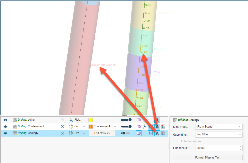
Once drilling data is visible in the scene, click on a borehole to view the data being displayed. You can also display the data associated with each interval by clicking on the Show text button (![]() ) in the shape list. Here, data display is enabled for two interval tables:
) in the shape list. Here, data display is enabled for two interval tables:
The Show trace lines button (![]() ) in the shape list displays all trace lines, even if there is no data defined for some intervals. The Filter trace lines option in the shape properties panel displays only trace lines for boreholes selected by a query filter. See the Query Filters topic for more information.
) in the shape list displays all trace lines, even if there is no data defined for some intervals. The Filter trace lines option in the shape properties panel displays only trace lines for boreholes selected by a query filter. See the Query Filters topic for more information.
Displaying Boreholes as Lines or Cylinders
You can display boreholes as lines or cylinders. You can also display the data associated with each segment. Here, the boreholes are displayed as flat lines:
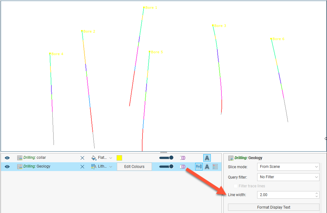
The width of the lines is set in the shape properties panel.
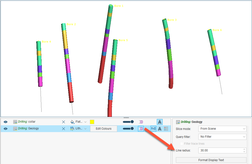
When the Make lines solid button (![]() ) is enabled, the boreholes are displayed as cylinders and the property that can be controlled is the Line radius:
) is enabled, the boreholes are displayed as cylinders and the property that can be controlled is the Line radius:
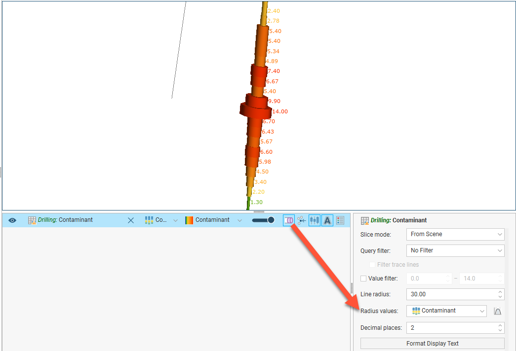
When numeric data is displayed, there is an additional option, to use a data column in the table for the cylinder radius:
When the log button (![]() ) is enabled, the log of values is used for the radius.
) is enabled, the log of values is used for the radius.
Hiding Lithologies
When lithology tables are displayed, you can hide some of the lithologies to help make better sense of the information in the scene. Click on the Edit Colours button in the shape list. In the window that appears, use the Show/Hide buttons (![]() ) to determine what segments are displayed:
) to determine what segments are displayed:
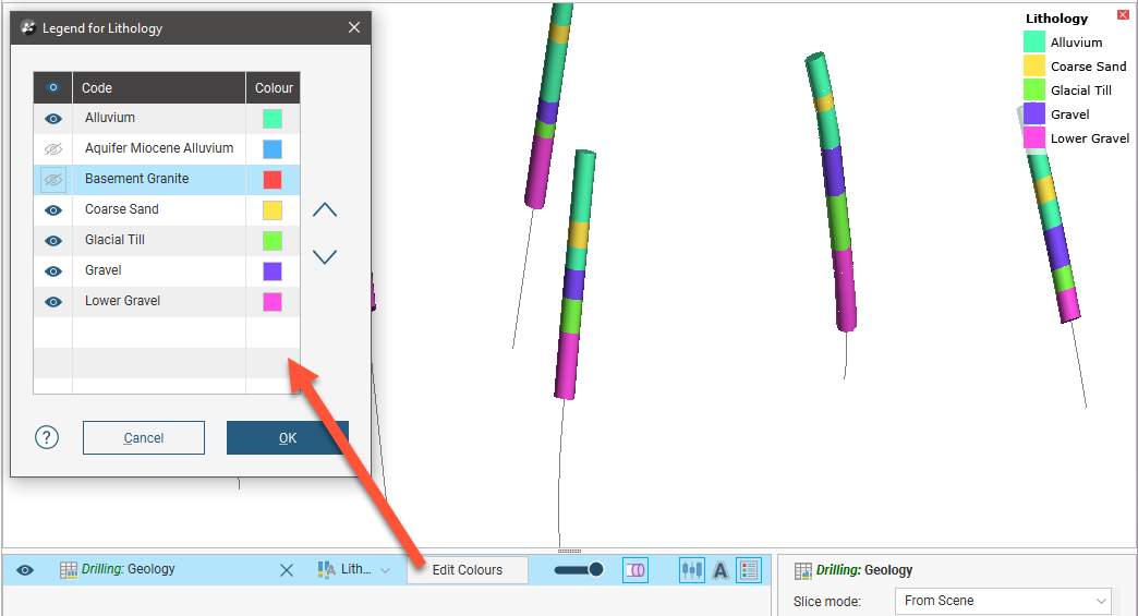
To select multiple lithologies, use the Shift or Ctrl keys while clicking. You can then change the visibility of all selected lithologies by clicking one of the visibility (![]() ) buttons.
) buttons.
Hiding lithologies in this way only changes how the data is displayed in the scene. Another way of limiting the data displayed is to use a query filter (see the Query Filters topic), which can later be used in selecting a subset of data for further processing.
Displaying a Legend
To display a legend in the scene, click the Show legend button (![]() ) for the table:
) for the table:
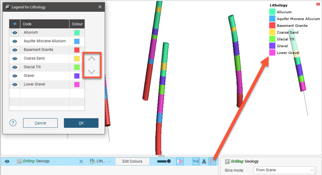
The legend in the scene will be updated to reflect lithologies that are hidden in the scene when you click Edit Colours and hide some lithologies.
To reorder the legend, click the Edit Colours button in the shape list to open the Legend window. Click on an item in the list, then use the arrows to move it up or down. The legend shown in the scene will be updated when you close the Legend window.
Changing Colourmaps
To change the colours used to display lithologies, click on the Edit Colours button in the shape list. In the window that appears, click on the colour chip for each lithology and change it as described in Single Colour Display.
Use the Shift or Ctrl keys to select multiple codes. This is useful for moving multiple codes up and down in the list.
You can also import a colourmap, which is described in Importing and Exporting Colourmaps.
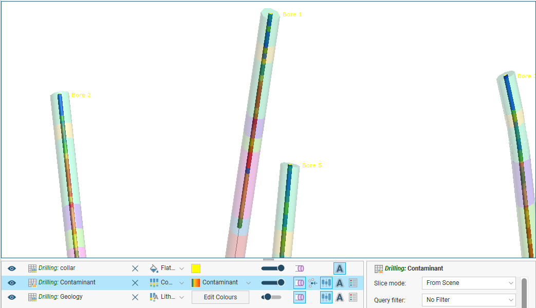
Viewing Multiple Interval Tables
When viewing multiple interval tables, use the line and point size controls and the transparency settings to see all the data at once. For example, here, the geology table has been made transparent to show the contaminant intervals inside:
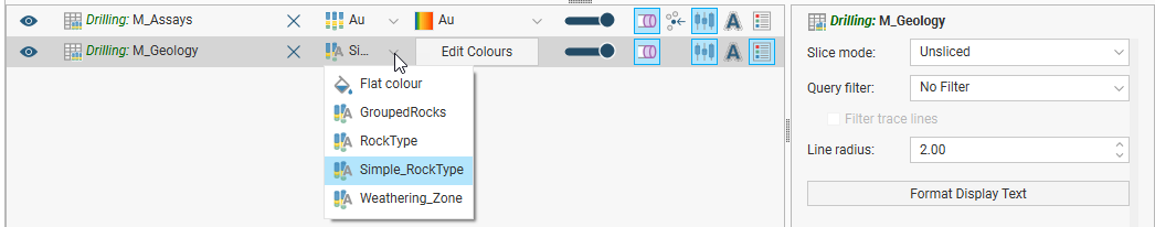
Selecting From Multiple Columns
When an interval table has more than one column of data, select the column to view from the view list:
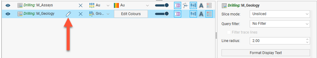
Some columns are editable, in which case you can click on the Edit button (![]() ) to start editing the table:
) to start editing the table:
Displaying Interval Data in the Scene
Boreholes can be displayed with the data associated with each segment. For example, in the scene below, contaminant values are displayed along the borehole:
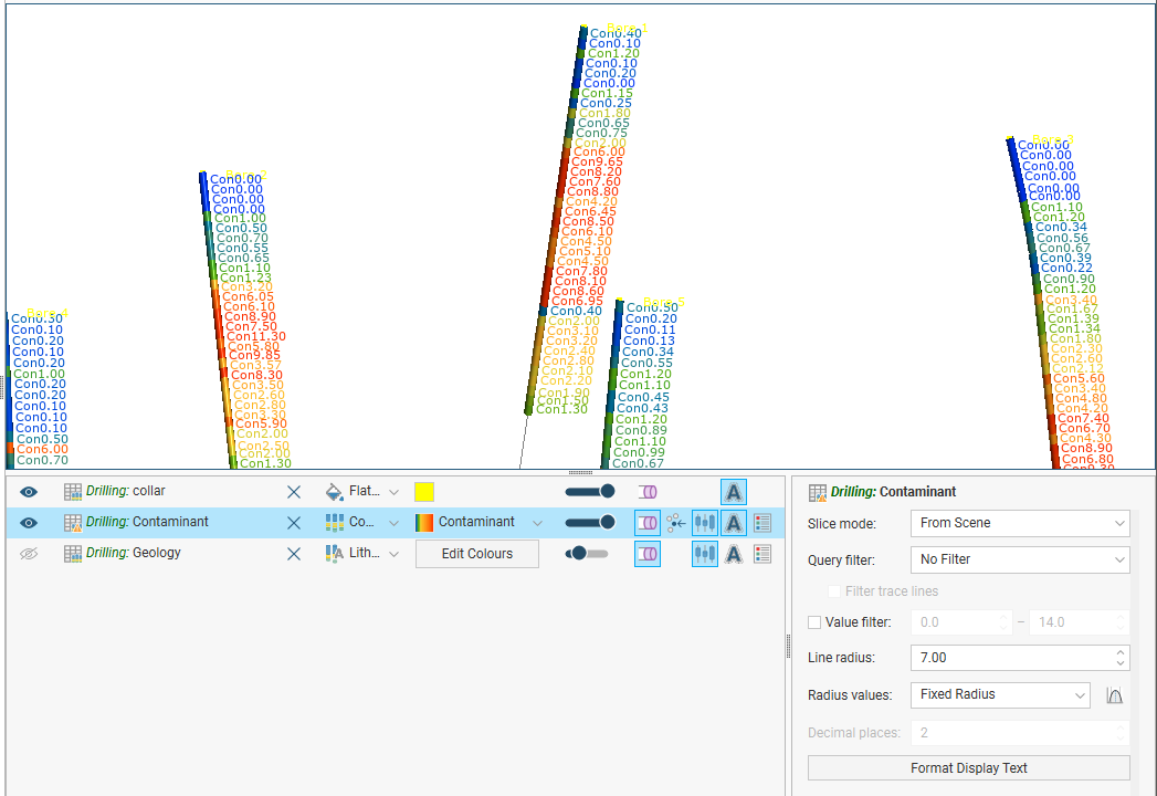
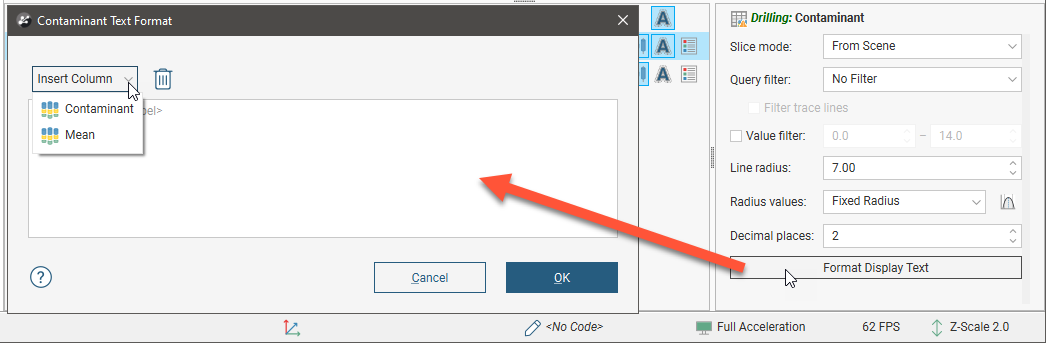
To view data in this way, select the table in the shape list, then click on the Format Display Text button. In the Text Format window, click Insert Column to choose from the columns available:
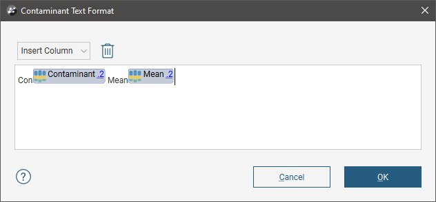
You can display multiple columns and add text:
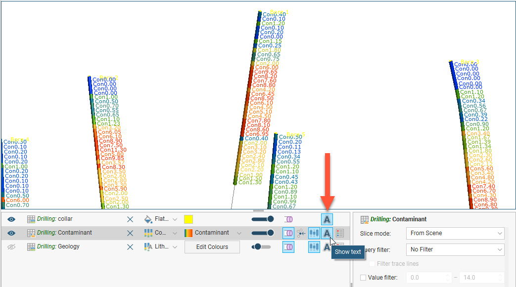
Click OK to update the formatting in the scene. You can conceal the formatting in the scene by clicking on the Show text button (![]() ) in the shape list:
) in the shape list:
Clear text formatting by clicking on the Format Display Text button, then on the Delete button (![]() ).
).
Displaying Borehole Traces
Adding the traces object (![]() ) to the scene can be useful in visualising the extent of drilling. You can change the colour used to display the traces, and they can be displayed as lines or cylinders. You can also display depth markers in the scene. To do so, click on the traces in the shape list and enable the Show depth marks option:
) to the scene can be useful in visualising the extent of drilling. You can change the colour used to display the traces, and they can be displayed as lines or cylinders. You can also display depth markers in the scene. To do so, click on the traces in the shape list and enable the Show depth marks option:
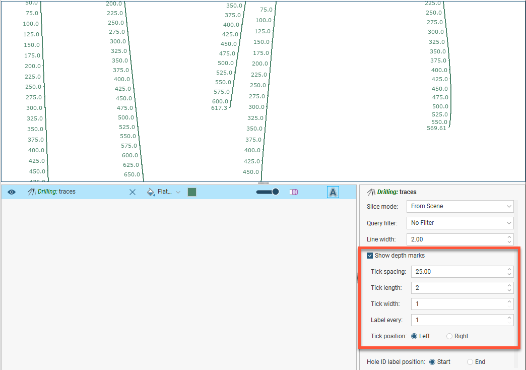
Depth markers can be displayed with or without text. Enable the Show text option ((![]() )) to display the depth values. This option also displays the hole ID, which can be displayed at the start or the end of the borehole.
)) to display the depth values. This option also displays the hole ID, which can be displayed at the start or the end of the borehole.
Displaying Borehole Graphs
Downhole numeric data can be displayed in the scene as a bar graph and downhole points data can be displayed as a line graph. To display downhole data in this way, add the graphs object (![]() ) to the scene. The Borehole Graph Style Manager will be displayed, showing the data columns available:
) to the scene. The Borehole Graph Style Manager will be displayed, showing the data columns available:
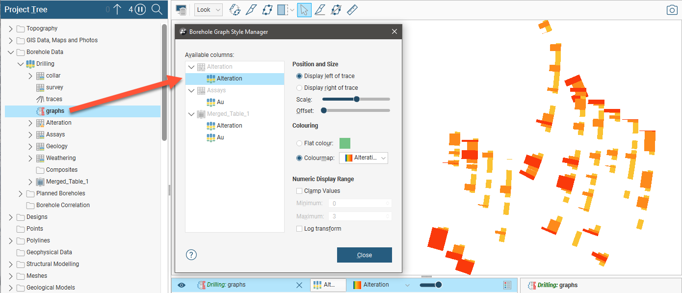
Data can be displayed to the right or the left of the borehole trace. Use the sliders to change the Scale and the Offset from the trace.
Data can be clamped, e.g. all values above the set maximum value will be set to the maximum value.
If there are negative values in the data, they will be displayed on the graph with a value of zero.
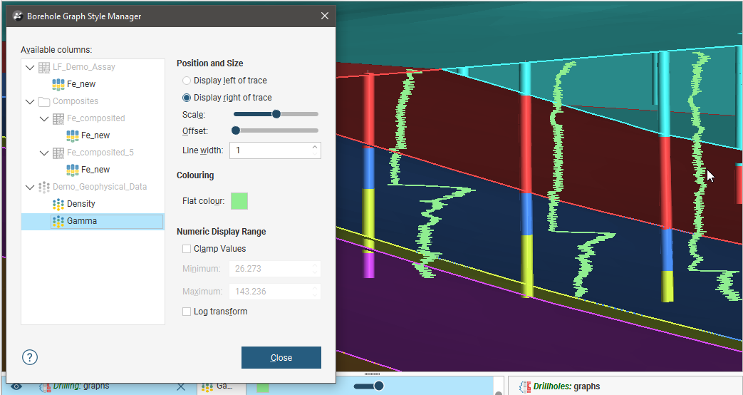
Downhole points can be displayed as a line, and you can change the Colouring, Scale and Offset of the line:
All changes made in the Borehole Graph Style Manager are automatically updated in the scene so you can experiment with the settings. Once you have closed the window, you can also change the Scale and Offset by clicking on the graphs object in the shape list:
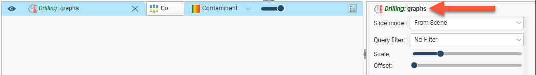
To select a different column to display, open the style manager by double-clicking on the graphs object in the project tree or select a new column from the shape list.
If you are working in a new project into which you have just imported boreholes, the Borehole Graph Style Manager will open when you add it to the scene. If the Borehole Graph Style Manager does not open when you add the graphs object to the scene, it is because the styles have already been set, perhaps by another user. You can change them by double-clicking on the graphs object.
Viewing Drilling Data Table Statistics
To view statistics on an interval table, right-click on the table in the project tree and select Statistics. The following options are available:
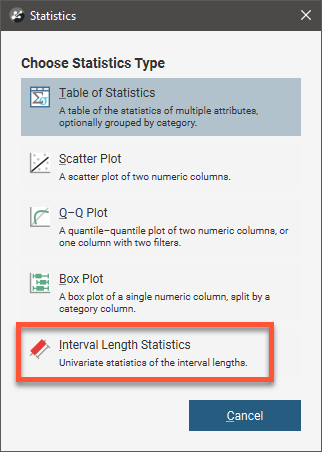
See the Statistics topic for more information on each option:
The Interval Length Statistics graph is a univariate graph, so for more information on the options available, see Univariate Graphs in the Statistics topic.
Right-click on a numeric column and select Statistics to open a univariate graph for that column.
Exporting Drilling Data
Changes made to the drilling data in Leapfrog Works only affect the Leapfrog Works database, not the original data files. You can export Leapfrog Works drilling data, which is useful if you wish to keep a copy of drilling data outside the project.
You can:
- Export all data in a drilling data set. See Exporting All Drilling Data.
- Export all data in a drilling data set in IFC format. See Exporting Drilling Data in IFC Format.
- Export only a single data table. See Exporting a Single Drilling Data Table.
These export options export the drilling data tables using To and From values to indicate location information. If you wish to export data with X-Y-Z values, extract points data using one of the following options:
- Extracting Contact Points from Drilling Data
- Extracting Intrusion Values from Drilling Data
- Extracting Interval Midpoints from Drilling Data
Then export the data object as described in Exporting Points Data.
Exporting All Drilling Data
To export all drilling data in a drilling data set, right-click on the data set and select Export. The Export Borehole Data window will appear:
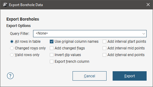
You can select whether the exported files includes all rows, only changed rows or only valid rows. You can also apply a query filter, if any have been defined for the drilling data set.
Once you have selected how you wish to export the data, click OK. The Export Borehole Data Files window will appear:
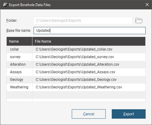
The list shows the files that will be created, one for each data table. Choose the Folder where the files will be saved, then enter a Base file name, which will be added to the front of each file name.
Click Export to save the files.
Exporting Drilling Data in IFC Format
Drilling data can be exported in the following IFC formats:
- IFC 2x3 (*.ifc)
- IFC 4.0 (*.ifc)
- IFC 4.3 RC3 (*.ifc)
Drilling data can also be exported in IFC format via the bulk exporter. See the Exporting Project Data to IFC topic for more information.
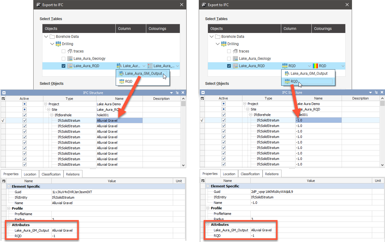
To export a drilling data set in one of the IFC formats, right-click on the data set and select Export > Export to IFC. In the window that appears, select the objects you wish to include, then enter a filename.
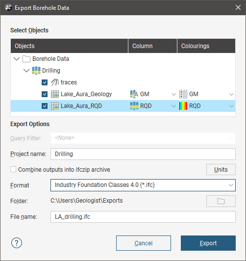
When an object has more than one colouring option available, you must choose which one you wish to use. If there is more than one colouring option, the other options will be exported as attributes. In this example, different columns are selected when drilling data is exported and the IFC structure is shown in BIMvision. Note that the selected column is exported as a SolidStratum type (in IFC 4.3 RC3) and both columns are included as attributes:
You can also:
- Combine outputs into an archive, in ifczip format
- Change the units used to export the data:
- Length can be in metres or feet
- Plane angle can be in radians or decimal degrees
Click Export to save the files.
See the Exporting Project Data to IFC topic for more information on the differences between the supported IFC formats.
Exporting a Single Drilling Data Table
To export a single drilling data table from a drilling data set, right-click on that table and select Export. The Export Borehole Data window will appear:
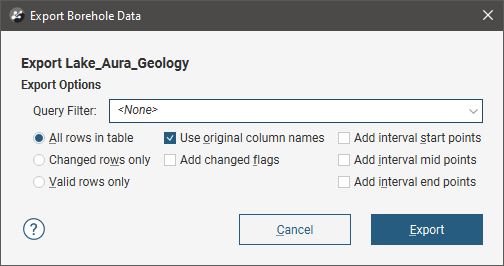
You can select whether the exported file includes all rows, only changed rows or only valid rows. You can also apply a query filter, if any have been defined for the drilling data set.
Once you have selected how you wish to export the data, click OK. You will be prompted for a filename and location.
Got a question? Visit the Seequent forums or Seequent support
© 2023 Seequent, The Bentley Subsurface Company
Privacy | Terms of Use