RBF Interpolants
If the data is both regularly and adequately sampled, different RBF interpolants will produce similar results. In practice, however, it is rarely the case that data is so abundant and input is required to ensure an interpolant produces geologically reasonable results. For this reason, only a basic set of parameters are required when an RBF interpolant is first created. Once the interpolant has been created, you can refine it to factor in real-world observations and account for limitations in the data.
The rest of this topic describes how to create and modify RBF interpolants. It is divided into:
- Creating an RBF Interpolant
- The RBF Interpolant in the Project Tree
- Interpolant Display
- RBF Interpolant Statistics
- Modifying an RBF Interpolant’s Boundary With Lateral Extents
- Changing the Settings for an RBF Interpolant
Creating an RBF Interpolant
To create an RBF interpolant, right-click on the Numeric Models folder and select New RBF Interpolant. The New RBF Interpolant window will be displayed:
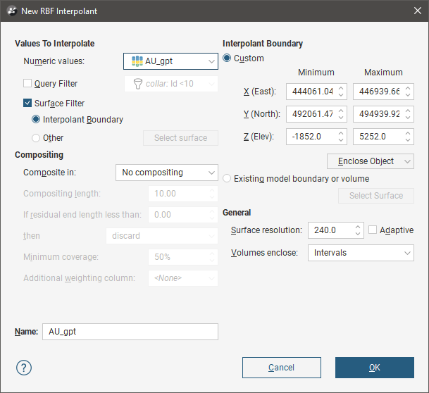
This window is divided into four parts that determine the values used to create the interpolant, the interpolant boundary, any compositing options and general interpolant properties.
If you are unsure of some settings, most can be changed later. However, the Numeric values object selected when the interpolant is created cannot be changed.
Values Used
In the Values To Interpolate part of the New RBF Interpolant window, you can select the values that will be used and choose whether or not to filter the data and use a subset of those values in the interpolant.
You can build an interpolant from either:
- Numeric data contained in imported drillhole data.
- Points data imported into the Points folder.
All suitable data in the project is available from the Numeric values list.
Applying a Query Filter
If you have defined a query filter and wish to use it to create the interpolant, select the filter from the Query filter list. Once the interpolant has been created, you can remove the filter or select a different filter.
Applying a Surface Filter
All available data can be used to generate the interpolant or the data can be filtered so that only the data that is within the interpolant boundary or another boundary in the project influences the interpolant. The Surface Filter option is enabled by default, but if you wish to use all data in the project, untick the box for Surface Filter. Otherwise, you can select the Interpolant Boundary or another boundary in the project.
You can use both the Query Filter option and the Surface Filter option together.
The Interpolant Boundary
There are several ways to set the Interpolant Boundary:
- Enter values to set a Custom boundary.
- Use the controls in the scene to set the Custom boundary dimensions.
- Select another object in the project from the Enclose Object list, which could be the numeric values object being interpolated. The extents for that object will be used as the basis for the Custom boundary dimensions.
- Select another object in the project to use as the Interpolant Boundary. Click the Existing model boundary or volume option and select the required object from the list.
Once the interpolant has been created, you can further modify its boundary. See Modifying an RBF Interpolant’s Boundary With Lateral Extents and Adjusting the Interpolant Boundary below.
Compositing Options
When numeric values from drillhole data are used to create an interpolant, there are two approaches to compositing that data:
- Composite the drillhole data, then use the composited values to create an interpolant. If you select composited values to create an interpolant, compositing options will be disabled.
- Use drillhole data that hasn’t been composited to create an interpolant, then apply compositing settings to the interpolated values. If you are interpolating values that have not been composited and do not have specific Compositing values in mind, you may wish to leave this option blank as it can be changed once the model has been created.
If you are interpolating points, compositing options will be disabled.
See Numeric Composites for more information on the effects of the Compositing length, For end lengths less than, Minimum coverage and Additional weighting column settings.
General Interpolant Properties
Set the Surface resolution for the interpolant and whether or not the resolution is adaptive. See Surface Resolution in Leapfrog Geo for more information on the effects of these settings. The resolution can be changed once the interpolant has been created, so setting a value in the New RBF Interpolant window is not vital. A lower value will produce more detail, but calculations will take longer.
The Volumes enclose option determines whether the interpolant volumes enclose Higher Values, Lower Values or Intervals. Again, this option can be changed once the interpolant has been created.
Enter a Name for the new interpolant and click OK.
Once you have created an RBF interpolant, you can adjust its properties by double-clicking on it. You can also double-click on the individual objects that make up the interpolant.
See also:
- Copying a Numeric Model
- Creating a Static Copy of a Numeric Model
- Exporting Numeric Model Volumes and Surfaces
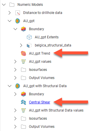
The RBF Interpolant in the Project Tree
The new interpolant will be created and added to the Numeric Models folder. The new interpolant contains objects that represent different parts of the interpolant:
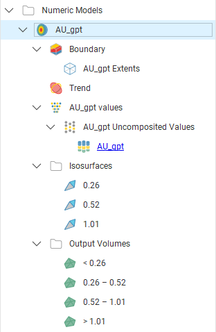
- The Boundary object defines the limits of the interpolant. See Adjusting the Interpolant Boundary.
- The Trend object describes the trend applied in the interpolant. See Changing the Trend for an RBF Interpolant.
- The points data values object contains all the data used in generating the interpolant. See Adjusting the Values Used.
- The Isosurfaces folder contains all the meshes generated in building the interpolant.
- The Output Volumes folder contains all the volumes generated in building the interpolant.
Other objects may appear in the project tree under the interpolant as you make changes to it.
Interpolant Display
Display the interpolant by:
- Dragging the interpolant into the scene or right-clicking on the interpolant and selecting View Output Volumes. Both actions display the interpolant’s output volumes.
- Right-clicking on the interpolant and selecting View Isosurfaces.
RBF Interpolant Statistics
You can view the approximated mean for each output volume by right-clicking on the interpolant and selecting Properties. Click on the Statistics tab:
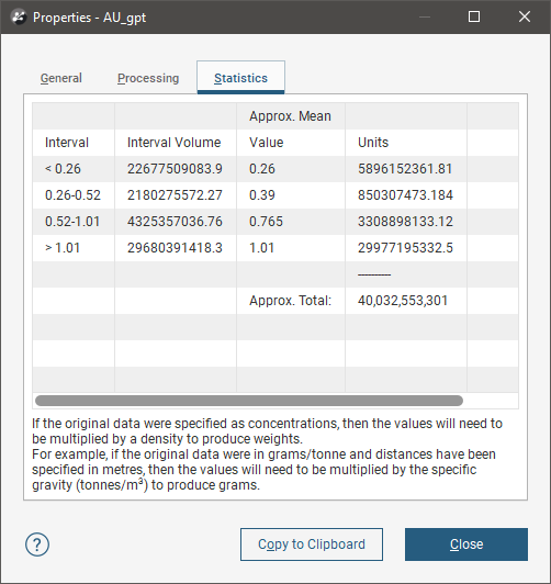
You can copy the information displayed in the Statistics tab to the clipboard for use in other applications.
Modifying an RBF Interpolant’s Boundary With Lateral Extents
RBF interpolants are created with a basic set of rectangular extents that can then be refined using other data in the project. These extents usually correspond to the ground surface and known boundaries. Creating extents can also be used to restrict modelling to a particular area of interest; for example, modelling can be restricted to a known distance from drillholes by applying a distance function as a lateral extent. Extents do not need to be strictly vertical surfaces and can be model volumes.
Creating Lateral Extents
To create an extent, expand the RBF interpolant in the project tree. Right-click on the Boundary object and select from the New Lateral Extent options. Follow the prompts to create the extent, which will then appear in the project tree under the interpolant’s Boundary object.
New extents are automatically applied to the boundary being modified. Leapfrog Geo usually orients a new extent correctly, with red presenting the inside face of the extent and blue representing the outside face. If this is not the case, you can change the orientation by right-clicking on the extent in the project tree and selecting Swap Inside.
Extent From a Polyline
You can create an extent from a polyline that already exists in the project or you can draw a new one. If you want to use an imported polyline, import it into the Polylines folder before creating the new extent.
To create a new extent from a polyline, right-click on the interpolant’s Boundary object and select New Lateral Extent > From Polyline. In the window that appears, select whether you will create a new polyline or use an existing one:
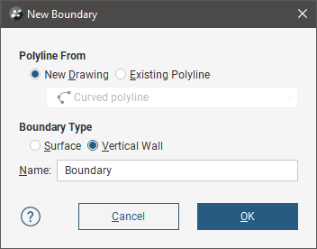
You can create the extent as a Vertical Wall or Surface. If you create the lateral extent as a Surface, you will be able to modify it using additional data, as described below. A lateral extent created as a Vertical Wall, however, cannot be modified.
Click OK to generate the new extent. If you have chosen to create a New Drawing, the drawing controls will appear in the scene and you can begin drawing, as described in Drawing in the Scene.
The new extent will appear in the project tree as part of the Boundary object.
If the surface generated does not fit the polyline adequately, you can increase the quality of the fit by adding more points to the polyline. See Drawing in the Scene for information on adding points to polylines.
Extents created from polylines can be modified by adding points data, GIS vector data and structural data. You can also add polylines and structural data to the extent. See Adding Data to an Extent, Editing an Extent With a Polyline and Editing an Extent With Structural Data for more information.
Extent From GIS Vector Data
GIS data in the project can be used to create a lateral extent for an RBF interpolant. Once the data you wish to use has been imported into the project, right-click on the interpolant’s Boundary object and select New Lateral Extent > From GIS Vector Data.
In the window that appears, select the data object you wish to use:
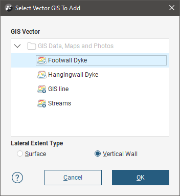
You can create the extent as a Vertical Wall or Surface. If you create the lateral extent as a Surface, you will be able to modify it using additional data, as described below. A lateral extent created as a Vertical Wall, however, cannot be modified.
If you select the Surface option, you can use the GIS data object with its own elevation data or projected onto the topography:
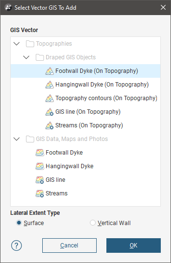
Using the On Topography option makes sense for GIS data as it is, by nature, on the topography. The On Topography option also mitigates any issues that may occur if elevation information in the GIS data object conflicts with that in the project.
Click OK to create the new extent. The new extent will appear in the project tree as part of the Boundary object.
Extents created from GIS data can be modified by adding points data, GIS vector data and structural data. You can also add polylines and structural data to the extent. See Adding Data to an Extent, Editing an Extent With a Polyline and Editing an Extent With Structural Data for more information.
Extent From Points
To create a new extent from points data, right-click on the interpolant’s Boundary object and select New Lateral Extent > From Points. The Select Points To Add window will be displayed, showing points data available in the project:
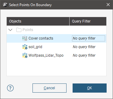
Select the information you wish to use and click OK.
The new extent will appear in the project tree as part of the Boundary object.
Extents created from points can be modified by adding points data, GIS vector data and structural data. You can also add polylines and structural data to the extent. See Adding Data to an Extent, Editing an Extent With a Polyline and Editing an Extent With Structural Data for more information.
Extent From Structural Data
Planar structural data can be used to create a lateral extent for an RBF interpolant. You can create a new structural data table or use a table that already exists in the project. If you want to use categories of structural data in creating the extent, use an existing table and create filters for those categories before creating the lateral extent.
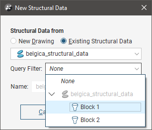
To start, right-click on the interpolant’s Boundary object and select New Lateral Extent > From Structural Data. The New Structural Data window will be displayed, showing structural data available in the project:
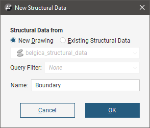
Select the New Drawing option to draw the structural data points directly in the scene.
Select the Existing Structural Data option to use a table in the Structural Modelling folder. With this option, you will be able to select from the categories available in the data table, if query filters have been created for those categories:
Click OK to generate the new extent. If you have chosen to create a New Drawing, the drawing controls will appear in the scene and you can begin drawing, as described in Creating New Planar Structural Data Tables. To share the new structural data table, right-click on it and select Share. The table will be saved to the Structural Modelling folder.
The new extent will appear in the project tree as part of the Boundary object.
Extents created from structural data can be modified by adding points data, GIS vector data and structural data. You can also add polylines and structural data to the extent. See Adding Data to an Extent, Editing an Extent With a Polyline and Editing an Extent With Structural Data for more information.
Extent From a Surface
To use a surface as lateral extent for an RBF interpolant, right-click on the interpolant’s Boundary object and select New Lateral Extent > From Surface. The Select Boundary window will appear, showing all the meshes that can be used as an extent:
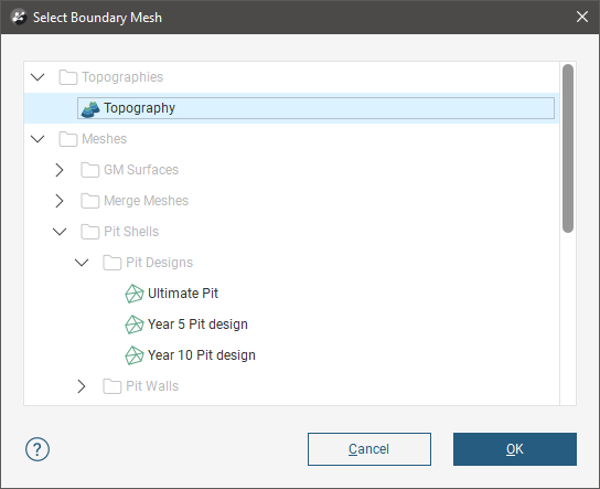
Select the required mesh and click OK. The extent will be added to the interpolant’s Boundary object.
You cannot modify an extent created from a mesh by adding data, editing with polylines or structural data or by applying a trend. However, the extent is linked to the mesh used to create it, and updating the mesh will update the extent.
Extent From Distance to Points
Leapfrog Geo can calculate the distance to set of points and use the resulting distance buffer as a lateral extent for an RBF interpolant. To create a new lateral extent from a distance buffer, right-click on the interpolant’s Boundary object and select New Lateral Extent > From Distance To Points. The Smoothed Distance Buffer window will appear:
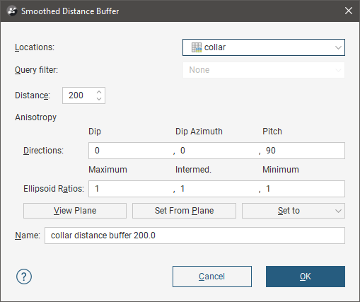
Select the Distance and set an Anisotropy, if required.
The Ellipsoid Ratios determine the relative shape and strength of the ellipsoids in the scene, where:
- The Maximum value is the relative strength in the direction of the green line on the moving plane.
- The Intermed. value is the relative strength in the direction perpendicular to the green line on the moving plane.
- The Minimum value is the relative strength in the direction orthogonal to the plane.
You can also use the Set to list to choose different options Leapfrog Geo has generated based on the data used to build the interpolant. Isotropic is the default option used when the interpolant is created.
Click OK to create the new extent, which will appear in the project tree as part of the Boundary object.
To change the extent’s settings, expand the interpolant’s Boundary object in the project tree and double-click on the extent. Adjust the Distance and Anisotropy, if required.
Extents created from a distance to points function can be modified by adding points data and GIS vector data. See Adding Data to an Extent.
Extent From a Distance Function
A distance function calculates the distance to a set of points and can be used to bound an RBF interpolant. You can use an existing distance function as a lateral extent or create a new one.
To use a distance function as a lateral extent, right-click on the interpolant’s Boundary and select New Lateral Extent > From Distance Function. If there are no distance functions in the project, you will be prompted to create a new one. See Distance Functions for information on defining and editing the distance function.
When there are already distance functions in the project, you will be prompted to choose between creating a new function or using an existing one:
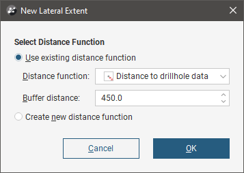
To use an existing function, select it from the list and set a Buffer distance. Click OK to create the lateral extent.
When you create a new distance function, it will be part of the interpolant’s Boundary object and will not be available elsewhere in the project. To share it within the project, expand the lateral extent in the project tree and right-click on the distance function. Select Share. The distance function will be saved to the Numeric Models folder.
To change the extent’s settings, expand the interpolant’s Boundary object in the project tree and double-click on the extent. Adjust the Distance and Anisotropy, if required.
Changing a Lateral Extent’s Settings
For lateral extents created from polylines, GIS data, points and structural data, you can change the extent’s settings by double-clicking on it in the project tree.
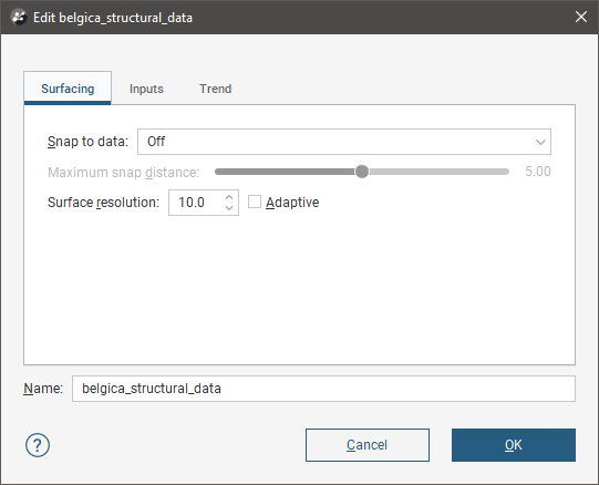
In the Surfacing tab, you can change surface resolution and contact honouring options, which are described below. In the Trend tab, you can apply a trend to the extent, which is described in Applying a Trend.
Surface Resolution
For RBF interpolants, the resolution of lateral extents is inherited from the settings in the interpolant’s Outputs tab, but the adaptive isosurfacer is automatically disabled. Enter a different Surface resolution value, if required, and tick Adaptive to enable the adaptive isosurfacer.
Contact Honouring
Often, surfaces should honour drillhole data and treat data objects such as polylines and GIS data as interpretations. For extents, the Snap to data setting in the Surfacing tab determines whether or not the extent honours the data used to create it. Options are:
- Off. The extent does not snap to the data used to create it. This is the default setting.
- All data. The extent snaps to all data within the Maximum snap distance, which includes drillhole data and any data added to the extent.
- Drilling only. The extent snaps to drillhole data and data objects derived from drillhole data within the Maximum snap distance, but not to other data used to modify the extent. For example, the extent will honour points data derived from drillhole data, but not points data imported into the Points folder.
- Custom. The extent snaps to the data objects indicated in the Inputs tab that are within the Maximum snap distance.
Take care in enabling snapping and in selecting what data the surface will snap to, as the more data you include, e.g. by setting a large Maximum snap distance or selecting All data for Snap to data, the greater the possibility that errors in the data or assumptions inherent in interpretations (e.g. polylines) will cause distortions in the meshes. If you do enable snapping, it is best to snap only to drilling data. See Honouring Surface Contacts for more information on these settings.
Whatever the setting, you can see what objects are snapped to by clicking on the Inputs tab.
If you need the extent to honour drillhole data but treat other data objects as interpretations, select Drilling only. To honour some data objects while treating others as interpretations, select Custom, then click on the Inputs tab to enable snapping for individual objects.
Applying a Trend
You can adjust an extent created from polylines, GIS data, points and structural data by applying a trend to it. To do this, add the extent to the scene. Next, double-click on the extent in the project tree and click the Trend tab.
Often the easiest way to apply a trend is to click on the Draw plane line button (![]() ) and draw a plane line in the scene in the direction in which you wish to adjust the surface. You may need to rotate the scene to see the plane properly.
) and draw a plane line in the scene in the direction in which you wish to adjust the surface. You may need to rotate the scene to see the plane properly.
The Ellipsoid Ratios determine the relative shape and strength of the ellipsoids in the scene, where:
- The Maximum value is the relative strength in the direction of the green line on the moving plane.
- The Intermed. value is the relative strength in the direction perpendicular to the green line on the moving plane.
- The Minimum value is the relative strength in the direction orthogonal to the plane.
Once you have adjusted the plane to represent the trend you wish to use, click the Set From Plane button to copy the moving plane settings.
The Set to list contains a number of different options Leapfrog Geo has generated based on the data used in the project. Isotropic is the default option used when the extent was created. Settings made to other surfaces in the project will also be listed, which makes it easy to apply the same settings to many surfaces.
Click OK to apply the changes.
See Global Trends in the Trends and Anisotropy topic for more information.
Adding Data to an Extent
Extents created from polylines, GIS data, points and structural data can be modified by adding points data objects, GIS vector data and structural data. Extents created from a distance to points function can be modified by adding points data and GIS vector data. To add data to an extent, right-click on the extent in the project tree and select the data type you wish to use from the Add menu.
- Points data. Select from the points data objects available in the project and click OK.
- GIS vector data. Select from the GIS vector data available in the project and click OK.
- Structural data. Select from the structural data tables available in the project. If the selected table has query filters defined, you can apply one of these filters by ticking Use query filter and then selecting the required filter from the list. Click OK to add the selected data to the extent. An alternative to adding an existing structural data table to an extent is to edit the extent with structural data. This is described in Editing an Extent With Structural Data below.
You can also add a polyline that already exists in the project. To do this, right-click on the extent in the project tree and select Add > Polyline. You will be prompted to choose from the polylines in the Polylines folder.
Editing an Extent With a Polyline
You can edit an extent using a polyline, which is described in Editing Surfaces With Polylines. A polyline used to edit an extent will be added to the project tree as part of the extent. To edit the polyline, right-click on it and select Edit Polyline or add it to the scene and click the Edit button (![]() ) in the shape list. If you wish to remove the polyline from the extent, right-click on it in the project tree and select Delete or Remove.
) in the shape list. If you wish to remove the polyline from the extent, right-click on it in the project tree and select Delete or Remove.
To add an existing polyline to a lateral extent, use the Add > Polyline option.
Editing an Extent With Structural Data
You can edit an extent using structural data, which is described in Editing Surfaces With Structural Data. A structural data table will be added to the project tree as part of the extent. To edit the table, right-click on it and select Edit In Scene or add it to the scene and click the Edit button (![]() ) in the shape list. If you wish to remove the table from the extent, right-click on it in the project tree and select Delete or Remove.
) in the shape list. If you wish to remove the table from the extent, right-click on it in the project tree and select Delete or Remove.
Removing an Extent from an Interpolant
If you have defined an extent and want to remove it from the interpolant, there are two options. The first is to right-click on the extent in the project tree and click Delete. This deletes the extent from the interpolant, but does not delete parent objects from the project unless they were created as part of the interpolant, e.g. a polyline used as a lateral extent but not shared within the project. Use this option only if you are sure you do not want to use the extent.
The second method is useful if you are making changes to the extent and do not want to recompute the interpolant with each change. Double-click on the interpolant’s Boundary object or double-click on the interpolant and click on the Boundary tab. The Boundaries part of the window lists all objects used as extents for the interpolant. Untick the box for extents to temporarily disable them in the interpolant. The interpolant will be reprocessed, but you can then work on the extent without reprocessing the interpolant. Disabled extents will be marked as inactive in the project tree.
Changing the Settings for an RBF Interpolant
To change the settings for an RBF interpolant, you can either double-click on the interpolant in the Numeric Models folder or right-click and select Open. When creating an RBF interpolant, only a basic set of parameters is used. The Edit RBF Interpolant window provides finer controls over these basic parameters so you can refine the interpolant to factor in real-world observations and account for limitations in the data.
For a multi-domained RBF interpolant, these parameters can be changed for the parent interpolant, and the trend, clipping, transformation and interpolation settings can be changed for the sub-interpolants.
Adjusting the Values Used
The Values tab in the Edit Interpolant window shows the values used in creating the interpolant and provides options for filtering the data. Although you cannot change the values used to create an interpolant, you can filter the values using the Query filter and Surface filter options.
You can adjust the values using a contour polyline or by adding points. Both options are available by expanding the interpolant in the project tree, then right-clicking on the values object:
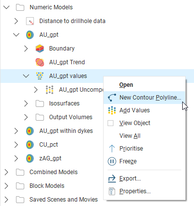
These options are described below in Adding a Contour Polyline and Adding Points.
To apply a query filter, tick the Query filter box in the Values tab and select the available queries from the list.
To change the object used as the Surface filter, select the required object from the list. Note that the list contains an object that defines the interpolant’s own boundary, which can be adjusted in the Boundary tab.
Adding a Contour Polyline
Adding a contour polyline is a useful tool for manually adjusting a surface to make it more geologically reasonable. To start adding a contour polyline, draw a slice where you wish to adjust the surface and decide what value you will assign to the contour line. Next, right-click on the values object and select New Contour Polyline. The next step is to choose whether you will draw a new polyline or use one already in the project:
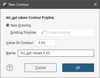
Only GIS lines, polylines imported into Leapfrog Geo or polylines created using the straight line drawing tool can be used to create contour lines.
Enter the value to be used for the contour and a name for it. Click OK. If you have chosen the New Drawing option, the new object will be created in the project tree and drawing tools will appear in the scene. Start drawing in the scene as described in Drawing in the Scene. When you have finished drawing, click the Save button (![]() ). The new contour will automatically be added to the interpolant and will appear in the project tree as part of the interpolant’s values object.
). The new contour will automatically be added to the interpolant and will appear in the project tree as part of the interpolant’s values object.
To change the value assigned to a contour polyline, double-click on the interpolant in the project tree. In the Values tab, contour polylines and their assigned values are shown in the User contour values table:
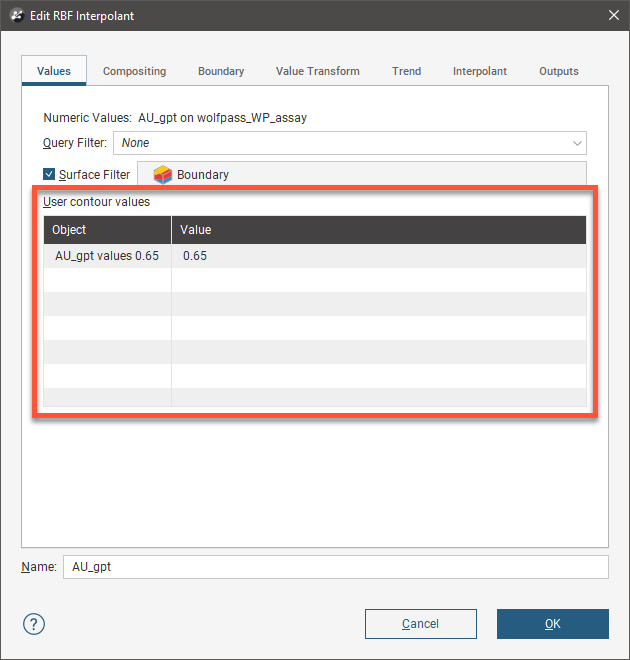
To change the value on a contour, click in the Value column and edit the entry.
To edit the polyline, right-click on it in the project tree and select Edit Polyline or add it to the scene and click the Edit button (![]() ) in the shape list. If you wish to remove a contour polyline from the interpolant, right-click on it in the project tree and select Delete or Remove.
) in the shape list. If you wish to remove a contour polyline from the interpolant, right-click on it in the project tree and select Delete or Remove.
Adding Points
To add points to an RBF interpolant, right-click on the values object in the project tree and select Add Values. Leapfrog Geo will display a list of all suitable points objects in the project. Select an object and click OK.
A hyperlink to the points object will be added to the values object in the project tree. To remove the points object, right-click on the points object and select Remove.
Compositing Parameters for an RBF Interpolant
When an RBF interpolant has been created from data that has not been composited, compositing parameters can be changed by double-clicking on the interpolant in the project tree, then clicking on the Compositing tab.
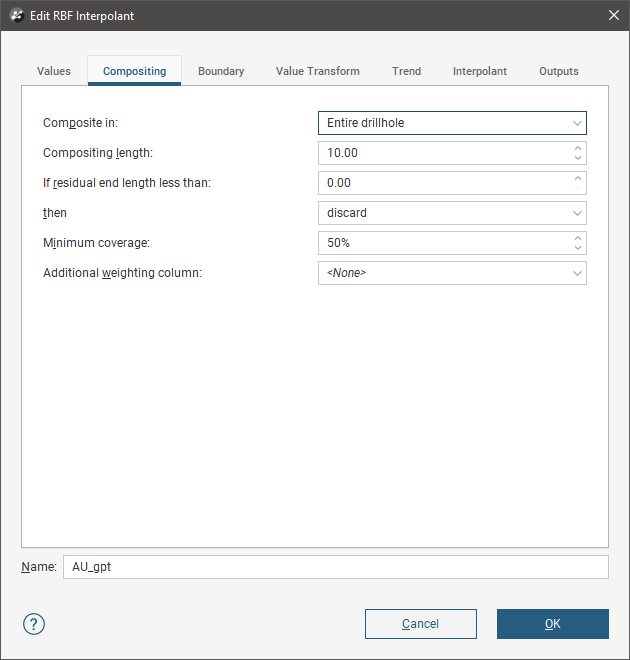
The Compositing tab will only appear for interpolants created from drillhole data that has not been composited.
You can composite in the entire drillhole or only where the data falls inside the interpolant boundary. See Numeric Composites for more information on the effects of the Compositing length, For end lengths less than and Minimum coverage settings.
Adjusting the Interpolant Boundary
See Modifying an RBF Interpolant’s Boundary With Lateral Extents above for information on creating and working with lateral extents.
To change an RBF interpolant’s boundary, double-click on the interpolant in the project tree, then click on the Boundary tab:
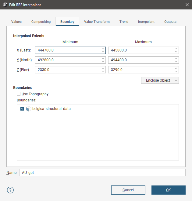
Controls to adjust the boundary will also appear in the scene.
Tick the Use Topography box to use the topography as a boundary. The topography is normally not used as a boundary for interpolants and so this option is disabled when an interpolant is first created.
The Boundaries list shows objects that have been used to modify the boundary. You can disable any of these lateral extents by unticking the box.
Lateral extents can be used to restrict modelling to a particular area of interest; for example, modelling can be restricted to a known distance from drillholes by applying a distance function as a lateral extent.
Clipping and Transforming Values for an RBF Interpolant
To clip data and apply a transformation to an RBF interpolant, double-click on the interpolant in the project tree, then click on the Value Transform tab:
![]()
The options for Transform Type are None and Log. Log uses a natural logarithm to compress the data values to a smaller range. This may be useful if the data range spans orders of magnitude. The function used is:
ln(x+s)+c
where s is the Pre-log shift and c is a constant. In order to avoid issues with taking the logarithm of zero or a negative number, Pre-log shift is a constant added to make the minimum value positive. The value of the pre-log shift will automatically be chosen to add to the minimum value in the data set to raise it to 0.001. This constant is then added to all the data samples. You can modify the value of the Pre-log shift, as increasing this value further away from zero can be used to reduce the effect of the natural logarithm transformation on the resultant isosurfaces.
Note that a further constant, c, is added to the natural logarithm of the data with the pre-log shift added to it. If there are any negative numbers that result from taking the natural log of the data, the absolute value of the most negative number is taken and added to all the transformed data results. This will raise the value of all the data so the minimum data value is zero. The value of c is chosen automatically and cannot be modified.
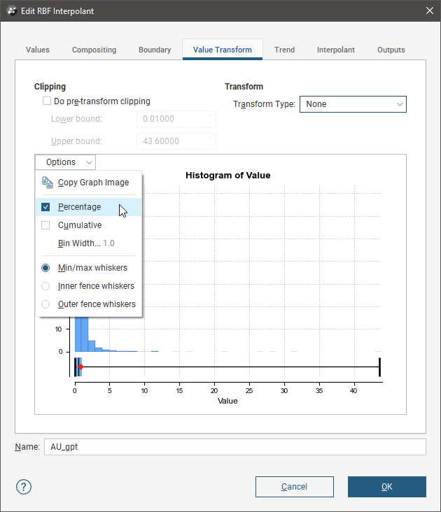
Click on the Options button to change the histogram’s display, including the Bin Width.
If you tick the Do pre-transform clipping option, you can set the Lower bound and the Upper bound to cap values that are too low or too high. For example, if you set the Upper bound from 14.00 to 10.00, grade values above 10.00 will be regarded as 10.00.
Changing the Trend for an RBF Interpolant
You can apply a global trend or a structural trend to an RBF interpolant. To do this, add the interpolant to the scene, then double-click on the interpolant in the project tree. Click on the Trend tab in the Edit RBF Interpolant window.
See:
Using a Global Trend
The easiest way to change the trend applied to an interpolant is using a global trend set from the moving plane.
Click View Plane to add the moving plane to the scene, then click on the plane to view its controls. You may need to hide part of the interpolant to click on the moving plane:
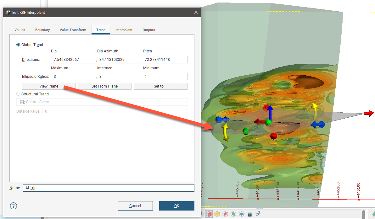
You can also use the Set to list to choose different options Leapfrog Geo has generated based on the data used to build the interpolant. Isotropic is the default option used when the interpolant is created.
The Ellipsoid Ratios determine the relative shape and strength of the ellipsoids in the scene, where:
- The Maximum value is the relative strength in the direction of the green line on the moving plane.
- The Intermed. value is the relative strength in the direction perpendicular to the green line on the moving plane.
- The Minimum value is the relative strength in the direction orthogonal to the plane.
Click OK to regenerate the interpolant and view changes.
Using a Structural Trend
You can also set the trend for an RBF interpolant from a structural trend. First, you must create or import the required mesh and create a structural trend. See Structural Trends in the Trends and Anisotropy topic for more information.
Once the structural trend has been created, add it to the interpolant by double-clicking on the interpolant in the project tree, then clicking on the Trend tab. Select the Structural Trend option, then select the required trend from the list:
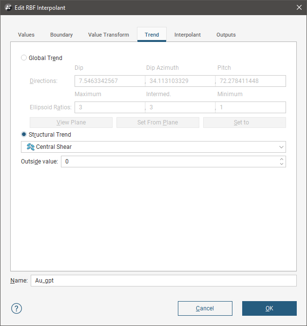
Click OK. The trend will be added to the interpolant and will appear as part of the interpolant, as shown:
When you apply a structural trend, you cannot use the Linear interpolant. See Interpolant Functions for more information.
Once a structural trend has been defined for the interpolant, you can edit it by clicking on the trend hyperlink in the project tree, then opening the structural trend applied to the interpolant. The Structural Trend window will appear. See Structural Trends in the Trends and Anisotropy topic for more information on the settings in this screen.
The structural trend information included as part of the interpolant is a link to the original structural trend. When you change the structural trend that is part of the interpolant, the changes are also made for the original structural trend.
When a structural trend that is Strongest along meshes or Blending is used, the interpolant will regress to the global mean trend away from the meshes. The global trend that will be used is set in the Global Trend tab for the structural trend.
Adjusting Interpolation Parameters
To adjust interpolation parameters for an RBF interpolant, double-click on the interpolant in the project tree, then click on the Interpolant tab:
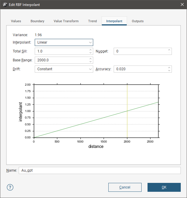
Two models are available, the spheroidal interpolant and the linear interpolant. See the Interpolant Functions topic for more information on the settings in this tab.
Output Settings for an RBF Interpolant
You can change the parameters used to generate RBF interpolant outputs by double-clicking on the interpolant, then clicking on the Outputs tab.
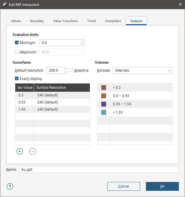
The Evaluation limits apply when interpolants are evaluated against other objects in the project. When the limits are enabled, all values outside the limits will be set to the Minimum and Maximum.
When Exact clipping is enabled, the interpolant isosurface will be generated without “tags” that overhang the interpolant boundary. This setting is enabled by default when you create an interpolant.
To add a new isosurface, click the Add button and enter the required value. To delete an isosurface, click on it in the list, then click the Remove button. You can also change the colours used to display the isosurfaces by clicking on the colour chips.
If you find that grade shells are overlapping, the resolution may be too coarse. Set Default resolution to a lower value or enable adaptive resolution in the Outputs tab. See Surface Resolution in Leapfrog Geo.
Got a question? Visit the Seequent forums or Seequent support