
Smooth Spectra
The RPS > Smooth Spectra option (geogxnet.dll(Geosoft.GX.Radiometrics.SmoothSpectra;Run)*) is an interactive tool for averaging and smoothing spectral radiometric data to improve the signal-to-noise ratio. Smoothing can be applied to a single line or to all selected lines in the database. The tool supports both NASVD and low-pass filtering, and includes eigenvalue/eigenvector analysis for optimal spectral reconstruction.
Smooth Spectra dialog options
|
Input channel |
Select the observed array channel containing the spectral radiometric data. Script Parameter: SPECTRO.SMOOTHING_INPUT_CHANNEL |
|
Output channel |
Enter a name for the output channel or choose from the available list. Default: Input channel_nasvd or Input channel_lp (suffix depends on the Method selection). Changing the default input channel will not automatically update the output channel name.
Script Parameter: SPECTRO.SMOOTHING_OUTPUT_CHANNEL |
|
Method |
Choose your preferred method for smoothing and noise reduction:
Script Parameter: SPECTRO.SMOOTHING_FILTER_METHOD [0 : NASVD; 1 : Low-Pass Filter] |
|
NASVD Parameters
Define the spectral energy window for eigenvector calculation – typical energy range (keV): 300 to 2810.
|
|
|
Start range (keV) |
Specify the start energy point. Default: 300 Script Parameter: SPECTRO.SMOOTHING_NASVD_START |
|
End range (keV) |
Specify the end energy point. Default: 2810 Script Parameter: SPECTRO.SMOOTHING_NASVD_END |
|
[Calculate Eigenvectors] |
Click to begin eigenvector calculation. The process runs in the background, allowing you to continue working or close the dialog. For further details, refer to the Application Notes below. Once complete, the Eigenvalues Tab becomes available. |
|
Number of eigenvectors |
After calculation, select how many eigenvectors to use for reconstruction from the dropdown. See Eigenvalue Visualization and Eigenvector Reconstruction for guidance. Script Parameter: SPECTRO.SMOOTHING_NASVD_EIGENVECTORS |
|
[Reset] |
You have the option to revisit your NASVD Start range/End range values. Click Reset to restore default NASVD range values and reset the dialog. See Eigenvalue Visualization and Eigenvector Reconstruction for guidance. |
|
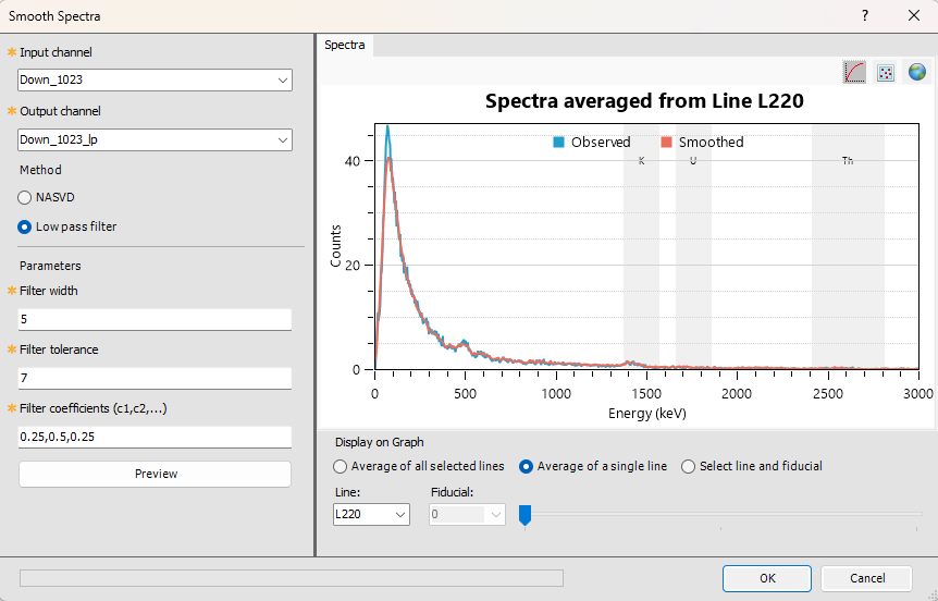
Low Pass Filter Parameters Specify the filtering parameters – enter custom values or use defaults to configure the filter. |
|
|
Filter width |
Define the bandwidth of the filter. Features wider than this value remain unchanged. Default: 5 Script Parameter: SPECTRO.SMOOTHING_LP_WIDTH |
|
Filter tolerance |
Set the amplitude threshold for noise removal. Default: 7 Script Parameter: SPECTRO.SMOOTHING_LP_TOLERANCE |
|
Filter coefficients (c1, c2,...) |
Enter comma-separated values (typically between 0 and 1; must be defined at discrete wavenumber increments). Default: 0.25,0.5,0.25 Script Parameter: SPECTRO.SMOOTHING_LP_COEFFICIENTS |
|
[Preview] |
Click to display the smoothed spectral graph in the right pane. See the Spectral Graph section below. |
Spectral Graph |
|
|
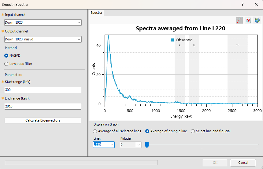
Observed Data |
The spectral plot provides a visual reference to help define energy ranges and understand how they span the gamma-ray spectrum. Once an input channel is selected, the right pane shows averaged spectral counts for Potassium (K), Uranium (U), and Thorium (Th). Shaded (labeled) rectangles indicate the energy windows for each element. Vertical grey dashed lines mark the NASVD start/end range and update dynamically. Graph Axes Display Controls Use the buttons on the top-right corner to scale the plot and display your spectral data:
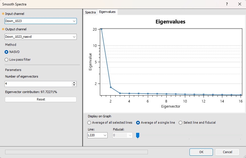
Left-click and hold to view X/Y values at the cursor location: Display Options Choose to view averaged spectra for:
|
|
NASVD-Smoothed Data |
Spectra TabOnce eigenvectors are calculated, the graph updates to display smoothed spectral counts for Potassium (K), Uranium (U), and Thorium (Th). Vertical grey dashed lines indicate the start and end of the selected spectral range. These lines adjust dynamically as the range is modified. The start and end values are also shown in the Jobs tab when the eigenvector calculation is executed.
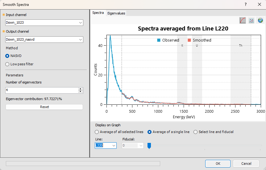
Smoothed profiles generated using NASVD spectral reconstruction are rendered within the dashed lines. This highlights that smoothing is applied exclusively to the portion of the spectrum inside the defined NASVD range. The final element on the far right of the array always includes all high-energy gamma rays, regardless of the array’s size. Impact of NASVD Smoothing The smoothed data closely follows the observed data until it enters the "smooth zone", after which it tapers toward observed values. To compare original and smoothed data, use the View Coincident Arrays tool. Eigenvalues TabNavigate to this tab to view the eigenvalue plot, which illustrates the relative contribution of each eigenvector to the overall data variance. The data is decomposed into a series of eigenvectors, each representing a principal direction of variance in the data. These are ranked by significance:
Early eigenvectors (typically the first few) exhibit a high signal-to-noise ratio and reflect meaningful structure in the data. Later eigenvectors tend to capture noise and contribute less to the reconstructed signal. (See Spectral Smoothing for more details.) Eigenvalue and Eigenvector Analysis You can interactively select how many eigenvectors to include in the reconstruction.
Refer to the Application Notes below for more details on interactive selection and visualization. |
|
To smooth your data using a low-pass filter, select the Low pass filter option, adjust the filter parameters, and click Preview. The graph will update to show smoothed spectral counts for Potassium (K), Uranium (U), and Thorium (Th). Smoothing is applied across the entire portion of the spectrum. This tool supports iterative refinement –experiment with different filter settings and click Preview to visualize the results. |
|
|
[OK] |
Once you are satisfied with the smoothing configuration and the quality of the filtered signal, click OK to save the changes to the output radiometric channel. The output will be stored as either an _nasvd or _lp database channel, depending on the method used. The OK button remains disabled until a smoothed spectrum has been generated.
|
 Toggle Y-axis between linear/logarithmic scale.
  Switch between line and point display.
 Zoom to full data extents.
 button again.
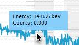
Application Notes
Compton scatter results from gamma rays losing energy as they collide with electrons along their trajectory. Thus, gamma rays below 300 keV are of different provenance and cannot be associated with radioelements of interest. The high end of the energy band (above 2810 keV) is too noisy and difficult to process.
Spectral Smoothing
Noise-Adjusted Singular Value Decomposition (NASVD) is a spectral noise-reduction technique designed to reduce statistical noise in gamma-ray spectra, significantly improving data quality. It applies a principal component analysis (PCA) to extract dominant spectral shapes (components) from raw input spectra. These components are then used to reconstruct spectra that retain most of the original signal while minimizing noise.
Because total counts are statistical in nature, they typically follow a Poisson distribution, where the variance equals the mean count rate in each energy bin. Prior to decomposition, NASVD normalizes the input spectra by the mean spectrum. It then uses all raw spectra to extract dominant spectral shapes—an approach analogous to PCA, which is widely used in multivariate analysis.
The principal components of a set of m spectra A are the eigenvectors of the covariance matrix ATA. These components are mutually orthogonal and arranged in descending order of their eigenvalues, which correspond to decreasing variance. The first component represents the average spectral shape across the dataset. When this component is subtracted from each spectrum, the second principal component captures the average shape of the residuals, and so on. Each eigenvalue reflects the variance associated with its corresponding component.
Observed spectra can be expressed as linear combinations of these components. Lower-order components capture the true signal, while higher-order components primarily represent uncorrelated noise. By reconstructing spectra using only the lower-order components, noise can be effectively suppressed. In practice, retaining 6 to 8 components is typically sufficient to preserve the signal.
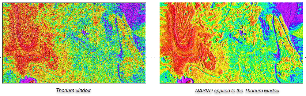
The most significant improvements are observed in the Uranium (U) window, followed by Thorium (Th), with the Potassium (K) window showing the least enhancement.
The illustration below presents an example of a NASVD-adjusted Thorium spectrum.
Eigenvector Calculation – Monitoring Progress in Project Explorer
You can track the progress of the eigenvector calculation while working on other tasks. The status (e.g., processing, completed, failed, cancelled) is visually indicated in the Jobs tab of the Project Explorer.
The process creates a new entry in the Jobs tab tree called Calculating NASVD Eigenvectors. The various steps of the process are listed under this node. Clicking the +/- icon expands or collapses the node.
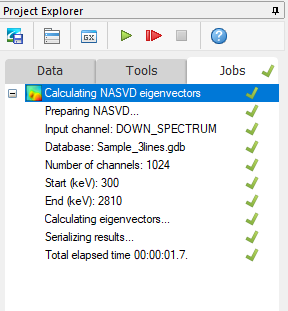
Refer to the Jobs Tab section in this topic for more details on monitoring progress and reporting results.
Eigenvalue Visualization and Eigenvector Reconstruction
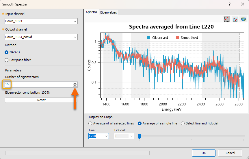
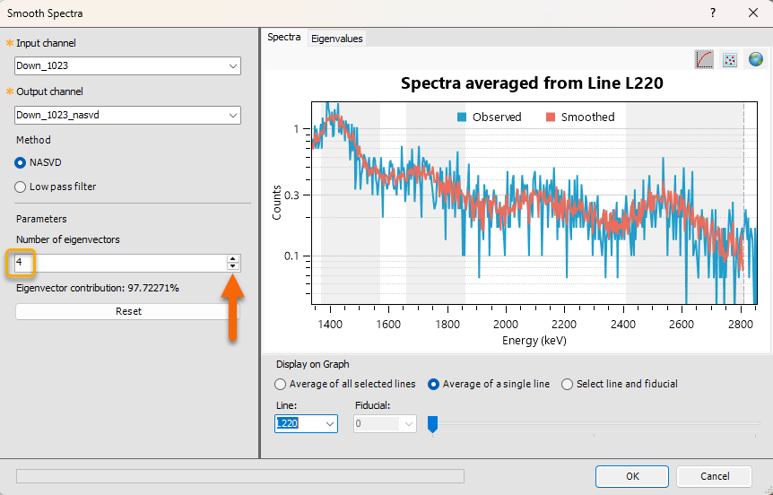
Interactive Selection and Visualization
- Use the stepper (up/down arrows) in the left pane to choose the number of eigenvectors to sum.
As more eigenvectors are added, the filtered signal (red curve) becomes noisier, and you can visually assess the trade-off between signal fidelity and noise.
In the example below, adding 16 eigenvectors seems to introduce unwanted noise, in comparison to a cleaner signal with the default selection of 4 eigenvectors.
Smoothing Range Configuration
- You can define the start and end points for the smoothing operation.
- This ensures that only the relevant portion of the data is processed—ignoring regions outside the area of interest.
Reconstruction and Refinement
- The Reset button allows you to reset the parameters, reprocess the eigenvectors based on updated parameters, and reconstruct the spectra.
- The Start range and End range fields become available and you can redefine the start and end points for the smoothing operation. This ensures that only the relevant portion of the data is processed—ignoring regions outside the area of interest.
Apply Spectral Smoothing
This tool enables iterative refinement and exploration of various smoothing configurations.
- Once you are satisfied with the selected number of eigenvectors and the quality of the filtered signal, click OK to apply the smoothing to the output radiometric channel.
- The resulting output—saved as the _nasvd database channel—will reflect the applied smoothing adjustments.
Acknowledgments
- As part of our radiometric data processing workflow, we’ve partnered with
Medusa has implemented the NASVD (Noise-Adjusted Singular Value Decomposition) method—a statistical technique that enhances gamma-ray spectra by reducing noise and improving signal clarity. This integration helps us deliver more accurate and reliable radiometric workflows and analysis.
Partner Integration: NASVD Method by Medusa Radiometrics
References
- [1] G. Erdi-Krausz et al. (2003), Guidelines for Radioelement Mapping Using Gamma Ray Spectrometry Data, IAEA-TECDOC-1363, International Atomic Energy Agency.
https://www-pub.iaea.org/MTCD/Publications/PDF/te_1363_web.pdf - [2] IAEA (1991), Airborne Gamma Ray Spectrometer Surveying, Technical Reports Series No. 323, International Atomic Energy Agency.
https://inis.iaea.org/collection/NCLCollectionStore/_Public/22/072/22072114.pdf
*GX.NET tools are embedded in the geogxnet.dll file located in the \Geosoft\Desktop Applications\bin folder. To run this GX interactively (outside the menu), first navigate to the bin directory and provide the GX.NET tool in the required format. See the Run GX topic for more guidance.
Got a question? Visit the Seequent forums or Seequent support
Copyright (c) 2025 Bentley Systems, Incorporated. All rights reserved.
Privacy | Terms of Use