
Smooth Spectra
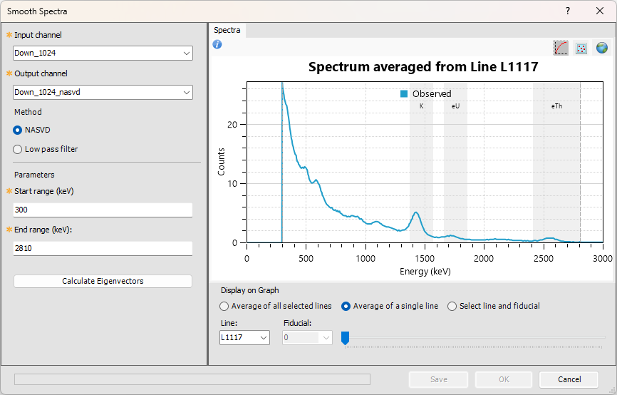
The RPS > Smooth Spectra option (geogxnet.dll(Geosoft.GX.Radiometrics.SmoothSpectra;Run)*) is an interactive tool for averaging and smoothing spectral radiometric data to improve the signal-to-noise ratio. Smoothing can be applied to a single line or to all selected lines in the database. The tool supports both NASVD and low-pass filtering, and includes eigenvalue and eigenvector analysis for optimal spectral reconstruction.
Smooth Spectra dialog options
|
Input parameters and previously calculated smoothed spectra are preserved and automatically reloaded when the dialog is reopened.
|
|
|
Input channel |
Select the array channel that contains the observed spectral radiometric data. Script Parameter: SPECTRO.SMOOTHING_INPUT_CHANNEL |
|
Output channel |
Specify the name of the channel that will store the smoothed spectral result, or select an existing channel from the list. By default, the output channel name is derived from the input channel:
Changing the input channel automatically updates the default output channel name.
Script Parameter: SPECTRO.SMOOTHING_OUTPUT_CHANNEL |
|
Method |
Select the smoothing and noise‑reduction method to apply to the input spectrum:
Switching between methods clears the graph in the right pane. If smoothing has already been calculated for the selected method, the system restores the results and displays the corresponding smoothed spectrum. Script Parameter: SPECTRO.SMOOTHING_FILTER_METHOD [0 : NASVD; 1 : Low-Pass Filter] |
|
NASVD Parameters
Define the spectral energy window for eigenvector calculation – typical energy range (keV): 300 to 2810.
|
|
|
Start range (keV) |
Specify the beginning of the energy range to process. Default: 300 Script Parameter: SPECTRO.SMOOTHING_NASVD_START |
|
End range (keV) |
Specify the end of the energy range to process. Default: 2810 Script Parameter: SPECTRO.SMOOTHING_NASVD_END |
|
[Calculate Eigenvectors] |
Click Calculate Eigenvectors to start the calculation. The process runs in the background, allowing you to continue working or close the dialog while it completes. When the calculation is complete:
If the selected data exceeds the processing limit, the system automatically switches to flight‑based grouping and displays a pre‑processing warning before the calculation begins.
For more information, see the Application Notes below. |
|
Number of eigenvectors |
After calculation, select the number of eigenvectors to use for reconstruction from the drop‑down list. See Eigenvalue and Eigenvector Analysis for guidance. Script Parameter: SPECTRO.SMOOTHING_NASVD_EIGENVECTORS |
|
[Reset] |
Click Reset to:
|
|
Low-Pass Filter Parameters Specify the filtering parameters – enter custom values or use the default values to configure the filter. |
|
|
Filter width |
Define the bandwidth of the filter. Features wider than this value remain unchanged. Default: 5 Script Parameter: SPECTRO.SMOOTHING_LP_WIDTH |
|
Filter tolerance |
Set the amplitude threshold for noise removal. Default: 7 Script Parameter: SPECTRO.SMOOTHING_LP_TOLERANCE |
|
Filter coefficients (c1, c2,...) |
Enter comma-separated values (typically between 0 and 1; must be defined at discrete wavenumber increments). Default: 0.25,0.5,0.25 Script Parameter: SPECTRO.SMOOTHING_LP_COEFFICIENTS |
|
[Preview] |
Click Preview to display the smoothed spectral graph in the right pane. See the Spectral Graph section below. |
Spectral Graph |
|
|
Observed Data |
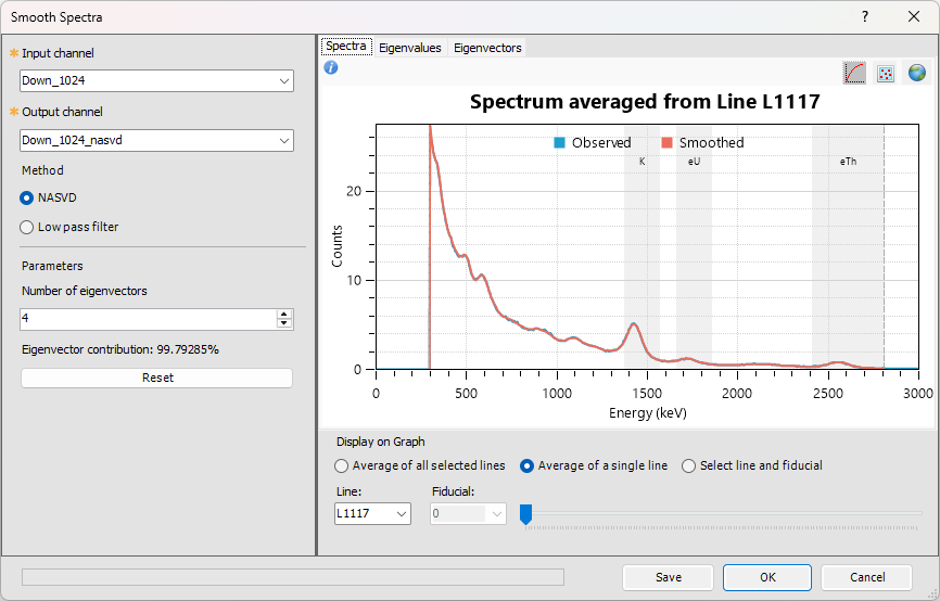
The spectral graph displays the averaged gamma-ray counts across the full energy spectrum. It is used to visually inspect overall spectral shape, identify key energy ranges, and understand how element responses (K, eU, eTh) are distributed. When an input channel is selected, the graph updates to display the averaged spectral counts. (For additional context, refer to Radioactive Decay and Gamma-Ray Emission in the Application Notes.) Changes made in the dialog update the graph dynamically. Axes
Shaded, labeled vertical bands indicate the expected energy windows for individual radioelements (K, eU, eTh). Grid Lines Grey grid lines are overlaid on the spectral plot for clarity:
NASVD Indicators When NASVD is selected:
If the averaged spectrum appears shifted along the energy axis, this can be corrected in a subsequent workflow. Display Controls (Graph Toolbar) The following controls are located in the upper‑right corner of the graph.
Display on Graph (Averaging Options) These options control how spectra are averaged and displayed on the graph.
When the selected line or fiducial changes:
Navigation and Interaction An information icon Zooming Use the following mouse interactions to explore the spectrum and inspect data values.
Panning
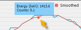
Data Inspection Reference Marker (Spectra tab only) As you move the cursor along the graph:
Viewing Data Values To inspect numeric values:
Because the marker snaps to true sample points, reported values may be slightly offset from the exact cursor position, depending on sampling density.
|
|
NASVD-Smoothed Data |
Finite-size radioelement responses generated over known radioelement calibration samples are used to fit the overall shape of the observed data. However, these sample responses lack the low-energy scatter present in airborne data, which originates from large lateral distances. As a result, the low-energy portion of the spectrum (< 300 keV) is omitted when decomposing the spectra. In the tool, NASVD decomposes the signal into a series of orthogonal principal components (eigenvectors), which are then ranked according to their corresponding magnitude (eigenvalues). By leveraging the correlations among radioelements, NASVD effectively reduces statistical error. This statistical approach is based on the premise that airborne spectra exhibit comparable shapes; subtle variations in photopeak amplitudes determine the relative contributions of individual radioelement sources. Spectra TabOnce the eigenvectors are calculated, the graph updates to display smoothed spectral counts across the full energy spectrum. Vertical grey dashed lines indicate the start and end of the selected spectral range. These lines adjust dynamically as the range is modified. The start and end values are also shown in the Jobs tab when the eigenvector calculation is executed.
Smoothed profiles generated using NASVD spectral reconstruction are rendered within the dashed lines. This highlights that smoothing is applied only to the portion of the spectrum within the defined NASVD range. The final element on the far right of the array always includes all high-energy gamma-ray counts, regardless of the array’s size. Impact of NASVD Smoothing The output spectra cover the same energy range as the input spectra. Within the specified energy range, the output spectra are smoothed; outside this range, the spectra remain unaltered. To compare the original and smoothed results, use the View Coincident Arrays tool. Eigenvalues TabNavigate to the Eigenvalues tab to view the eigenvalues plot, which shows the relative contribution of each eigenvector to the overall data variance. This plot helps guide the selection of an appropriate number of eigenvectors for spectral reconstruction (see also Eigenvector Selection and Spectral Smoothing). All mouse interactions available in the Spectra tab are also supported here. Hover over the information icon
Eigenvalue and Eigenvector Analysis The data is decomposed into a series of eigenvectors, each representing a principal direction of variance. Eigenvectors are ranked by eigenvalue magnitude:
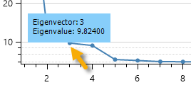
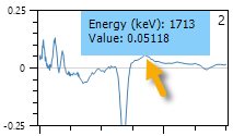
Early eigenvectors typically have a high signal‑to‑noise ratio and represent meaningful spectral structure. In contrast, later eigenvectors increasingly capture noise and contribute little to improving the reconstructed signal. This behaviour appears in the eigenvalues curve as a sharp initial decrease followed by a gradual flattening (see also Spectral Smoothing). A key decision point is identifying where the eigenvalues curve begins to flatten (that is, approaches an asymptote). In the example shown above, the curve flattens around eigenvector 3–4, indicating diminishing returns from including additional components. Higher‑order eigenvectors beyond this point primarily introduce noise rather than improving the reconstructed signal. The point at which the curve flattens typically indicates an appropriate value to enter in the Number of eigenvectors control in the left pane. Inspecting Individual Eigenvectors Click on a point in the Eigenvalues plot to display the corresponding eigenvector index and its eigenvalue.
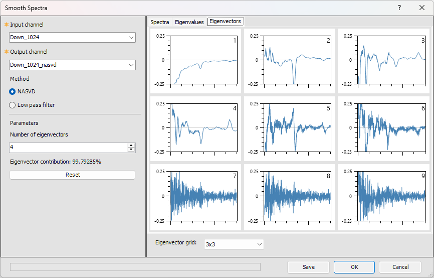
This allows for closer inspection of individual components before determining the number of eigenvectors to use in the reconstruction. Eigenvectors TabCheck the Eigenvectors tab to identify NASVD eigenvectors that represent meaningful signals when combined, and to disregard those that primarily represent noise. Survey reports often include these plots to support the chosen number of eigenvectors representing the actual signal. Eigenvector Plot Layout Eigenvectors are shown in a grid format, where each plot represents an individual eigenvector component. The order in which they are plotted (from left to right and from top to bottom) is governed by the decreasing magnitude of their eigenvalues. Typically:
The objective is to select enough eigenvectors to capture the real signal while minimising noise. Visual Consistency Across Plots To ensure valid visual comparison, all eigenvector plots share the same display settings:
Axes Definition
Using a common, clipped Y‑axis range preserves the main structure of each eigenvector while preventing distortion from large or anomalous values. This makes it easier to compare shapes and relative magnitudes across components. Interacting with the Eigenvectors View
|
|
Low-pass Filtered Data |
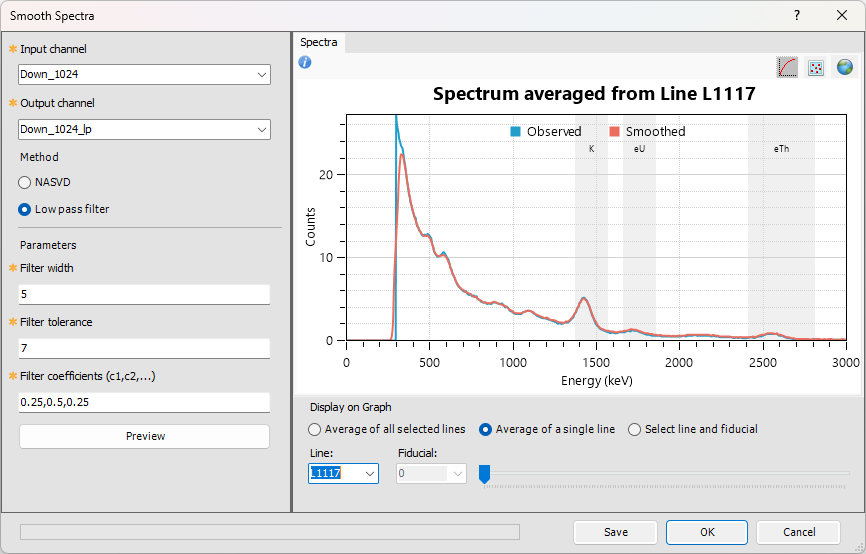
To apply spectral smoothing using a low-pass filter, select the Low pass filter option, adjust the filter parameters, and click Preview. The graph refreshes to display the smoothed spectral counts across the entire energy spectrum. This tool supports iterative refinement—experiment with different filter settings and click Preview to visualize the results. |
|
|
|


 in the upper‑left corner of the graph provides a quick summary of available zooming and panning controls.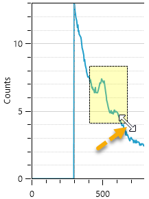
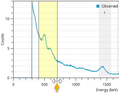
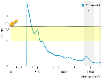
 at the top of the plot.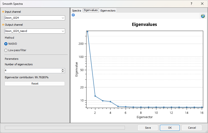
|
[Save] |
The Save button remains disabled until a smoothed spectrum has been successfully generated. Click Save to commit the current smoothed spectrum to the database while keeping the dialog open. The default output is saved as either an _nasvd or _lp channel in the database, depending on the smoothing method used. If a channel with the same name already exists, a confirmation dialog prompts you to confirm that you want to overwrite it. After saving, the Smooth Spectra dialog remains open, and the newly generated output channel is immediately displayed in the active database view.
|
|
[OK] |
The OK button also remains disabled until a smoothed spectrum has been successfully generated. Click OK to commit the smoothed spectrum to the database and exit. As with Save, the default output is stored as either an _nasvd or _lp channel, and a confirmation prompt appears if you attempt to overwrite an existing channel with the same name. |
Application Notes
Compton scatter occurs when gamma rays lose energy through collisions with electrons along their path. As a result, gamma rays below approximately 300 keV originate from different processes and cannot be reliably associated with radioelements of interest. At the upper end of the energy band (above 2810 keV), the spectrum becomes too noisy to interpret or process effectively.
Selecting this range correctly is essential, as data containing non-radiation-related components can compromise or even disable processes such as Principal Component Analysis. It is good practice to set the lower limit beyond the leftmost spectral peak and to set the upper limit so that it excludes the array element containing the cosmic count.
Radioactive Decay and Gamma Ray Emission
Potassium concentrations in rocks and soils are commonly estimated using gamma‑ray spectrometry, which detects the 1461 keV gamma rays emitted by the radioactive isotope potassium-40 (40K). Unlike 40K, which decays directly to a stable daughter isotope, uranium‑238 (238U) and thorium-232 (232Th) decay through long chains of intermediate, unstable daughter products.
For gamma-ray spectrometry, the energies associated with these decay series are identified through their most prominent daughter isotopes:
-
238U → 214Bi (bismuth)
-
232Th → 208Tl (thallium)
Characteristic gamma‑ray energy peaks — most notably the 1765 keV line from 214Bi and the 2615 keV line from 208Tl — serve as markers for the uranium and thorium decay chains. The intensities of these emissions are then scaled to estimate concentrations of uranium and thorium, reported as equivalent uranium (eU) and equivalent thorium (eTh).
Spectral Smoothing
Noise-Adjusted Singular Value Decomposition (NASVD) is a spectral noise-reduction technique designed to reduce statistical noise in gamma-ray spectra, significantly improving data quality. It applies a Principal Component Analysis (PCA) to extract dominant spectral shapes (components) from raw input spectra. These components are then used to reconstruct spectra that retain most of the original signal while minimising noise.
Because total counts are statistical in nature, they typically follow a Poisson distribution, where the variance equals the mean count rate in each energy bin. Prior to decomposition, NASVD normalises the input spectra by the mean spectrum. It then uses all raw spectra to extract dominant spectral shapes—an approach analogous to PCA, which is widely used in multivariate analysis.
The principal components of a set of m spectra A are the eigenvectors of the covariance matrix ATA. These components are mutually orthogonal and arranged in descending order of their eigenvalues, which correspond to decreasing variance. The first component represents the average spectral shape across the dataset. When this component is subtracted from each spectrum, the second principal component captures the average shape of the residuals, and so on. Each eigenvalue reflects the variance associated with its corresponding component.
Observed spectra can be expressed as linear combinations of these components. Lower-order components capture the true signal, while higher-order components primarily represent uncorrelated noise. By reconstructing spectra using only the lower-order components, noise can be effectively suppressed. In practice, retaining 6 to 8 components is typically sufficient to preserve the signal.
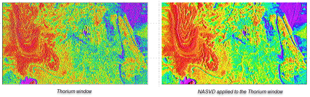
The most significant improvements typically appear in the uranium window, followed by thorium, while the potassium window shows the least change.
The illustration below shows an example of a NASVD-adjusted thorium spectrum.
Eigenvector Calculation – Monitoring Progress in Project Explorer
You can track the progress of eigenvector calculation while working on other tasks. The status (e.g., processing, completed, failed, cancelled) is visually indicated in the Jobs tab in Project Explorer.
The process creates a new entry in the Jobs tab tree called Calculating NASVD Eigenvectors. The steps of the process are listed under this node. Click the +/- icon to expand or collapse the node.
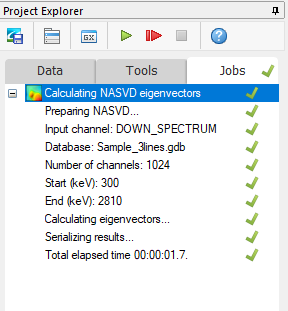
Refer to the Jobs Tab section in this topic for more details on monitoring progress and reporting results.
NASVD_Coeff Definition
NASVD_Coeff represents the relative contribution of each NASVD component at every measurement point (spectrum).
The array stores the 16 amplitudes (coefficients) of the 16 computed and sorted eigenvectors:
-
Each element corresponds to one eigenvector
-
Element 0 = first eigenvector
-
Element 1 = second eigenvector
-
and so forth.
Each array element represents the spatial expression of its corresponding eigenvector, where higher values indicate a greater contribution to the spectrum.
The computed eigenvectors remain in memory while you determine how many components to use to reconstruct smoothed spectra.
Selecting the Number of Components
Choosing the appropriate number of eigenvectors for smoothing is a key challenge:
-
Too few components → may remove real signal
-
Too many components → may leave hindering residual noise
Eigenvalue and eigenvector plots provide valuable overall guidance but may not clearly indicate the correct cutoff:
-
Some datasets do not show a clear inflection point in the eigenvalue plot.
-
Adjacent eigenvectors may appear visually similar in eigenvector plots.
-
Components with low overall importance (i.e., low eigenvalues) may still contain meaningful localised signals within the survey.
The NASVD_Coeff channel provides a complementary, spatially aware method that can be used alongside eigenvalues and eigenvectors for more refined interpretation.
Identifying Spatial Structure in Components
NASVD_Coeff can reveal locally significant components that may otherwise be overshadowed by overall statistical noise.
Start by creating grids from individual elements of the NASVD_Coeff array (for example, using the Grid Multiple Channels tool) and examining them side by side:
-
Coherent structure across multiple NASVD_Coeff grids → indicative of a spatially meaningful signal
-
Random or noisy appearance → indicative of a noise-dominated component
As a practical guideline, select the lowest-numbered eigenvector that shows coherent structure across multiple NASVD_Coeff grids.
An eigenvector may have a low eigenvalue but still exhibit strong, localised patterns or isolated features within the survey.
In large survey areas, these localised features may be overshadowed by the overall expression of the dataset.
Validating Component Selection
As noted by Hovgaard & Grasty [3], generally a small number of components captures most of the spectral information. However, further examination of the spectral coefficients can provide greater confidence that subtle but real signals are not discarded.
Strong, coherent structure in coefficient grids may also indicate distinct spatial regions or clusters, suggesting the dataset could benefit from segmented processing or grouping.
Recalculation Behaviour
When eigenvectors are recalculated, or when you click OK or Save, the NASVD_Coeff channel is automatically updated to reflect the current decomposition and component selection.
If you need to retain previous results, make a copy of the existing NASVD_Coeff channel before proceeding.
Terminology
In spectral component analysis (Hovgaard & Grasty, 1997 [3]), amplitude represents the amount or strength of a spectral component (eigenvector) present in a measured spectrum at a given measurement point.
-
Eigenvectors — spectral components
-
Eigenvalues — the amount of variance accounted for by each component
-
NASVD_Coeff (coefficients) — amplitude of each component at each measurement point
NASVD Smoothing – Large Dataset Handling and Pre-Processing Warning
NASVD eigenvector calculations are limited to a maximum of 500,000,000 elements, defined as:

If the selected dataset exceeds this limit, the system automatically switches to flight-based grouping and displays a pre‑processing warning before the calculation begins.
Pre‑Processing Warning Dialog
The warning dialog explains why flight-based grouping is required and provides the following information:
-
Processing limit – NASVD can process up to 500,000,000 elements in a single calculation.
-
Dataset size – The total number of elements in the selected data.
-
Record count – The current number of records (rows), and the maximum allowed before grouping is required.
-
Required reduction – The percentage reduction needed to bring the dataset below the processing limit.
You are then prompted to choose how to proceed:
-
OK – Continue with flight-based grouping
-
The dataset is grouped by flight.
-
Each flight is processed and smoothed independently.
-
Eigenvector plots are not displayed.
-
Eigenvalues shown in the Eigenvalues tab are averaged across all processed flights.
-
-
Cancel – Stop processing and return to the Smooth Spectra dialog.
To avoid flight-based grouping, you can:
Select a smaller subset of lines or flights.
Reduce the dataset size by compressing spectral data into fewer windows.
Post‑processing Behaviour with Flight-Based Grouping
When flight-based grouping is used, the output has the following characteristics:
-
The Eigenvectors tab is hidden.
-
The Eigenvalues tab displays an averaged profile titled “Eigenvalues – Averaged Flights”.
-
The NASVD_Coeff channel and related output channels are populated only for the processed flights.
Interactive Spectral Smoothing Using Eigenvectors
Eigenvector Selection and Visualization
Use the stepper controls (up/down arrows) in the left pane to select the number of eigenvectors to include in the reconstruction.
As additional eigenvectors are added:
-
The filtered signal (red curve) begins to exhibit increased noise.
-
You can visually assess the trade-off between signal fidelity and noise reduction.
-
In many cases, a small number of eigenvectors (for example, four) produces a cleaner, more stable spectrum than larger selections.
Reconstruction and Refinement
The Reset button allows you to reset the parameters and reprocess the eigenvectors based on the updated values. The Start range and End range fields then become available, allowing you to redefine the smoothing boundaries. This ensures that only the region of interest is processed, while areas outside this range remain unaffected.
Apply Spectral Smoothing
This tool supports iterative exploration and refinement of smoothing configurations.
- After selecting an appropriate number of eigenvectors and verifying the quality of the filtered signal, click Save to apply the smoothing. Click OK to apply the smoothing and close the dialog.
- The output is saved as a new radiometric channel with the _nasvd suffix, reflecting the applied NASVD smoothing parameters.
Acknowledgments
- As part of our radiometric data processing workflow, we’ve partnered with
Medusa has implemented the NASVD (Noise-Adjusted Singular Value Decomposition) method—a statistical technique that enhances gamma-ray spectra by reducing noise and improving signal clarity. This integration helps us deliver more accurate and reliable radiometric workflows and analysis.
Partner Integration: NASVD Method by Medusa Radiometrics
References
- [1] G. Erdi-Krausz et al. (2003), Guidelines for Radioelement Mapping Using Gamma Ray Spectrometry Data, IAEA-TECDOC-1363, International Atomic Energy Agency.
https://www-pub.iaea.org/MTCD/Publications/PDF/te_1363_web.pdf - [2] IAEA (1991), Airborne Gamma Ray Spectrometer Surveying, Technical Reports Series No. 323, International Atomic Energy Agency.
https://inis.iaea.org/collection/NCLCollectionStore/_Public/22/072/22072114.pdf - [3] J. Hovgaard, R.L. Grasty (1997), Reducing Statistical Noise in Airborne Gamma-Ray Data through Spectral Component Analysis, Proceedings of Exploration 97, Fourth Decennial Internal Conference on Mineral Exploration 1997, pp. 753–764.
*GX.NET tools are embedded in the geogxnet.dll file located in the \Geosoft\Desktop Applications\bin folder. To run this GX interactively (outside the menu), navigate to the bin directory and specify the GX.NET tool in the required format. See the Run GX topic for more guidance.
Got a question? Visit the Seequent forums or Seequent support
Copyright (c) 2026 Bentley Systems, Incorporated. All rights reserved.
Privacy | Terms of Use